Features
What Fairbeam does
Feature overview: modeling, simulation, exports, example projects and their simulated results.
Feature overview
-
Ribbon-based designer
A one-row ribbon, a collapsible navigation tree, properties and dock, and a Python side panel. Bricks, cylinders, spheres, cones, tori, wires, polygons and extrusions; draw bricks in 3D, extrude a picked face, booleans, one Transform dialog, shortcuts, Undo, Redo and Save As.
-
Import a VBA macro
Imports supported commands from CST-compatible VBA macros and history lists, with a report of unsupported or changed operations. Review the report and imported model before running.
-
Parameters and checks
Dimensions and frequencies can use named parameters. Live checks explain detected problems and block known invalid setups, including designs without an excited port. Convergence still needs to be checked after running.
-
Start templates and examples
Start from a half-wave dipole, a quarter-wave monopole, an open-ended waveguide, a printed sleeve dipole or a two-port microstrip line, or pick an example from a searchable list, which now includes a 2-element collinear and a 5-element Yagi for 867 MHz.
-
Import PCB artwork
Home › Import PCB turns DXF, Gerber and Excellon files into a design;
fairbeam import-pcbdoes the same from the command line. -
Automatic meshing
Auto mode picks the mesh settings for each design, and every field can be overridden. Thin PCB copper is meshed as sheets, and converted examples keep their own mesh lines. In the dipole and patch checks below, resonance differs from converged hand-tuned meshes by about 0.1% or less.
-
Mesh convergence
Mesh convergence studies refine automatic meshes and compare resonance, |S11| and Dmax against tolerances, stopping at convergence or the configured run limit. Also available through fairbeam converge.
-
Run quality and one-click fixes
Run-quality warnings and one-click fixes flag common problems. With calibrated waveguide-port power, the horn example has about 99.3% raw radiation efficiency at 10 GHz; its lossless-normalized result is 100%.
-
Parameter sweeps
Queue checked sweep sequences over up to six parameters and compare selected runs, up to eight at a time, in one plot.
-
Goal-driven optimizer
Goals such as f0, |S11| at a frequency, bandwidth, Dmax or |Sij| limits, over as many parameters as you vary. Secant, Nelder–Mead, Bayesian, CMA-ES, particle swarm, genetic and trust-region searches, with live progress; the best result is kept to open, apply or save.
-
Multi-port S-parameters
One openEMS run per driven port gives the full S-matrix of filters, dividers, couplers and arrays, with reciprocity and passivity checks, a picker for any Sij, a Smith chart per port and Touchstone
.sNpexport. -
Results with markers
Result tabs: S-parameters, impedance, VSWR, Smith chart, efficiency and patterns, with markers for resonances and bandwidth, hover read-outs and your own markers. Runs are compared by the parameters that differ; Copy data and CSV in dB, phase, Re/Im or magnitude/phase.
-
Result summaries and comparison
Headline numbers for each run in the tree and the Runs table, and Tables › Summary. A comparison table lists the parameters that differ between runs; copy it or save it as CSV.
-
2D and 3D field maps
The Field map tab shows E and H planes as heat maps with a read-out and the model's outline. Phase and Animate play a time-harmonic animation of the field, in 2D and in the 3D view.
-
Far field, currents, beams
View directivity, gain, realized gain, polarization, currents and steered array patterns. Optional radiation and total efficiency curves are computed after the solver finishes; additional post-processing time depends on the model and frequency count.
-
GPU engines
Optional openEMS GPU builds support Metal on Apple silicon and CUDA on NVIDIA GPUs under Windows. Documented patch solver times were 1.6 s versus 10.6 s on an M5 Pro and 2.6 s versus 52.9 s on a Ryzen 9 7900X with RTX 3060, using the recorded runtimes. GPU startup preference can be changed; CPU remains available.
-
VBA macro, drawings, fabrication
Export a CST-compatible VBA macro for supported geometry and settings; check the reconstructed model in the target program. Export Touchstone, CSV, drawings, figures, a PDF report and preview fabrication files.
-
Desktop app
For macOS and Windows, in English or Turkish (General settings › Language, native menus included, with a Decimal separator setting), with Save As, and a question before closing unsaved work. First start installs Python and openEMS for your user account; projects live in Documents/Fairbeam, and updates are offered in the app.
Example projects
19 simulated projects come with the app and are listed in the browser demo. Six of them:
- Pyramidal horn, WR-90
- An optimum-gain horn fed by a TE10 waveguide port, with PML boundaries: 15.5 dBi at 10 GHz and |S11| below −16 dB from 8 to 12 GHz.
- Axial-mode helix
- A Kraus helix, seven turns at 13° pitch over a square ground plane: right-hand circular, 11.6 dBi at 2.4 GHz, an axial ratio of 0.9 dB on boresight and the cross-polarized LHCP 26 dB lower.
- Minkowski fractal patch
- The fractal edge lengthens the current path: 30 × 30 mm of copper resonates at 2.324 GHz, below the 32 × 40 mm plain patch at 2.453 GHz on the same substrate, at the price of bandwidth (0.8 %).
- Wilkinson divider
- Three ports and one lumped 100 Ω resistor: an equal split with S21 = S31 = −3.09 dB. One openEMS run per driven port gives the full S-matrix.
- Branch-line coupler
- A 90° hybrid: −3.21 and −2.99 dB to the two outputs at 2.40 GHz, 90.0° apart, with the reciprocity and passivity of the four-port matrix checked.
- Stepped-impedance low-pass
- Alternating wide and narrow line sections: the −3 dB point lands at 2.356 GHz, 5.2 % below the ideal line cascade, because the steps themselves add capacitance.
The files, as they come out
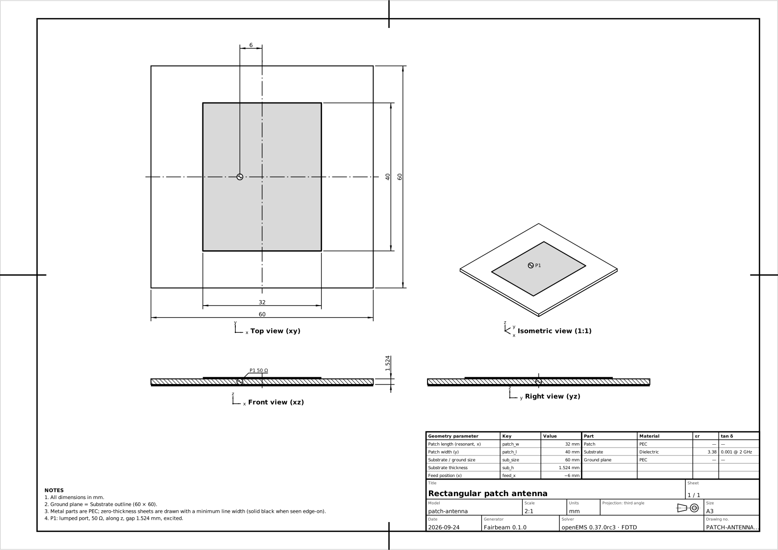
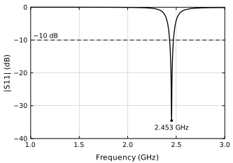
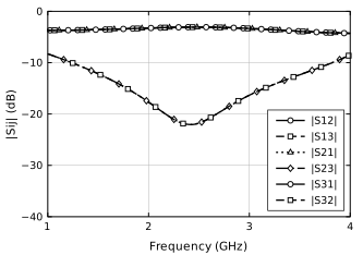
Simulation results and recorded solver times
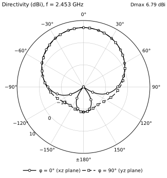
Validation
| Check | Fairbeam | Reference |
|---|---|---|
| Dipole Dmax | 2.13–2.15 dBi | 2.11 dBi (theory) |
| Patch resonance | 2.455 GHz | 2.513 GHz (TL model), −2.3 % |
Dipole: three lengths, 50 to 66 mm, end criterion −60 dB. Patch: converged mesh, against a transmission-line model. Details and commands in the validation notes of the repository.
Solver time in seconds
| Model | Cells | Apple M5 Pro | Ryzen 9 7900X | |||
|---|---|---|---|---|---|---|
| CPU | GPU | 4 threads | 24 threads | CUDA | ||
| Patch antenna, −60 dB | 0.26 M | 10.6 | 1.6 | 52.9 | 49.9 | 2.6 |
| 4 × 1 patch array (4 runs) | 0.43 M | – | 14.2 | 874 | 686 | 25.1 |
| Sierpinski monopole | 2.0 M | 12.0 | 2.7 | 61.1 | 65.7 | 3.4 |
For the documented same-timestep Windows CPU / macOS Metal comparisons, S-parameter magnitudes above −30 dB agree within 0.1 dB and Dmax within 0.004 dB. Other comparisons have different bounds; see the benchmark notes. The optional GPU engine is a separate beta fork of openEMS.
Circuits and arrays
| Check | Fairbeam | Reference |
|---|---|---|
| Microstrip line Z0 | 48.3 Ω | 50.0 Ω (Hammerstad) |
| Wilkinson split S21 = S31 | −3.09 dB | −3.01 dB (ideal) |
| Branch-line S21 / S31 | −3.21 / −2.99 dB | −3.01 dB each |
| Low-pass −3 dB point | 2.356 GHz | 2.485 GHz (ideal) |
| 4×1 array S11 / S22 | −23.5 / −17.0 dB | 4 GPU runs |
For the recorded 100 Ω Wilkinson example, output match and isolation are −18.4 and −22.0 dB. Resistor checks agree within 0.1% in their tested range; the divider discrepancy remains unresolved. The documented branch-line output phase difference is 90.0° at 2.40 GHz, and the low-pass cutoff is 5.2% below the ideal-line model.
Optimizer
| Task | Result | Cost |
|---|---|---|
| Dipole to f0 = 2.40 GHz | 2.4000 GHz | 2 evaluations |
| Wilkinson: all ports ≤ −20 dB, S23 ≤ −25 dB | 82 Ω | 3 evaluations |
| Wilkinson: S23 ≤ −35 dB | 73 Ω | 4 evaluations |
The isolation resistor went from the textbook 100 Ω to 73 Ω in the documented optimization; with all ports driven, 73 Ω gives S23 = −39.9 dB and every port matched below −24 dB.
Automatic mesh
| Model | Automatic | Converged |
|---|---|---|
| Dipole | 2.4182 GHz | 2.4198 GHz, −0.07 % |
| Patch antenna | 2.4525 GHz | 2.4550 GHz, −0.10 % |
What to expect
- Development preview
- The designer, the solver pipeline and the results work end to end. The file formats are versioned (
fairbeam.design/1for designs,fairbeam.project/1for results); breaking changes bump the version. - VBA macro export not yet validated
- The exported CST-compatible VBA macro and the macro import are not validated for every command or physical port formulation; the macro import reports the commands that it skips or changes. Check an exported model in the target program before relying on it.
- Fabrication files not yet validated
- Selected fabrication fixtures are parsed back and checked against their geometry to 1 µm. These preview exports are not fab-validated. Check each export in an independent viewer and review clearances, footprints and fabrication tolerances before ordering.
- Wilkinson output match: open question
- The 100 Ω Wilkinson example has output match and isolation below the analytical expectation. Tested resistor fixtures agree within 0.1%; the remaining layout and mesh discrepancy needs further investigation.
- Windows installer not code-signed, macOS 27+
- The managed macOS solver requires macOS 27+ on Apple silicon. Windows installers are not code-signed and may trigger SmartScreen. Linux currently uses a source setup with compatible openEMS and CSXCAD versions; see the tested configuration and limits. The macOS app is signed with a Developer ID and notarized by Apple.
- Licenses
- Fairbeam is GPL-3.0-or-later; openEMS is GPL-3.0-or-later and CSXCAD LGPL-3.0-or-later. The source code is on GitHub: ismailakdag/fairbeam (opens in a new tab). Project files are plain data produced by your own models.
Planned and finished work is on the roadmap.