The designer is Fairbeam's visual modeling workspace, laid out as a one-row ribbon over the 3D view, the navigation tree on the left, the properties of the selection on the right, a dock with the checks, the parameters and the progress of a run at the bottom, and a status bar. The results of a run open as tabs beside the 3D view. You draw or add shapes, give them materials, place ports, set up the simulation, run openEMS and read the results without leaving the model.
A design is a data file, <name>.design.json, not Python. Everything else in Fairbeam (the CLI,
sweeps, the optimizer, the Run panel) treats a design like any model, and you can export it as a
Python model file at any time.
The designer needs the run server (fairbeam serve, see Run server and Run panel). The
desktop app (DESKTOP.md (opens in a new tab)) starts it for you. The public demo is read-only and has no
designer.
Start screen
The start screen opens when the run server is reachable. It has three parts:
- New design: a name (filled in from the starting point until you type your own) and a starting point. The file name follows from the name
(
Dual-band patch→dual_band_patch.design.json). "Empty design" gives a band (f0 × 0.6 to 1.4, MUR boundaries, −50 dB end criterion), copper (no dielectric: Materials › Add dielectric copies FR4 or another library material when a substrate is needed), and no geometry. The starters are small parametric designs, grouped as Basic antennas, Printed and Circuits (see Starters below). Create and open the designer makes the file and opens it. Import VBA macro… makes a design from a CST-compatible VBA macro or history list (.bas,.mcs,.txt) instead (see Importing a VBA macro); Import PCB artwork… does so from DXF or Gerber files (see Importing PCB artwork). - Your designs: search by name, ID, or filename, sort by name or recent modification, and star favorite designs. Favorites appear first and the favorites filter and sort choice are remembered in this browser. Older entries without a modification timestamp use their name as a fallback. Open one in the designer. Right-click a saved design (or press Shift+F10 while its row is focused) to Rename its display name or Show in File Explorer in the desktop app. Renaming keeps its file, ID and existing results, and offers Undo on Start; save an open design's edits first. The bin icon deletes a design after a confirmation; the file moves to the model history folder, so it can be restored. A design file that does not open (damaged, or made by a newer Fairbeam) stays in the list, grayed, with the reason.
- Python models and Examples: open a model in the Run panel, or an example with its results (in Examples mode). Open as new design… next to an example makes an editable design of your own from it. The runs of your designs are not listed here: they open under the design (see Running and results).
The footer's Send feedback links open the public issue tracker in your browser; see Feedback.
Start lists your own Python models first, then the bundled examples' models, marked example,
read-only: a click opens one in the Run panel (a bundled one asks to copy it or to run it as it is),
and its copy button makes an editable design of it. On Start, the header's Run a Python model…
scrolls to this list. The Examples card groups the examples like the header's picker, with their
bands and mesh sizes. A new design's file name is the ASCII form of its name; a name that is a
bundled example's ID gets a number (Patch antenna is saved as patch_antenna_2.design.json), as the
line under the Name field shows. Save as… (Home ribbon › Project, the header's More menu,
Shift+Ctrl+S or ⇧⌘S where the browser leaves it to the page, and File › Save As in the desktop app)
saves a copy of the open design under a new name.
The header's Start · Design · Examples switch moves between the start screen, the designer and the examples:
The header's More menu keeps secondary actions available with arrow-key navigation and Escape.
Open result or design file… is available there and through desktop File → Open: a result
file (.json of a run) opens in Examples; a design file (.design.json, e.g. Export › Current
design JSON from a colleague) is created as a new design in the workspace, under a free file name
from its name, and opened in Design. Dropping either on the window does the same. Opening a design
lists its saved runs under Results in the tree; select a run to view it without opening a file
manually.
On narrow windows the tree and properties panels share one overlay slot so they do not cover
both sides of the canvas at once. Resizing back restores the independently remembered desktop
panel choices. General Settings and About take focus whenever opened; dialogs contain Tab,
isolate the background, and restore focus when closed. Escape closes the top dialog unless an
inner control handles it first.
Design owns its runs. They are listed under Results in the navigation tree and open in place: the 3D view shows the run's geometry with its pattern or surface currents, the dock its plots.
Examples is the viewer described in the README (opens in a new tab) and How results are computed, on the example projects: the bundled ones, with their results ready, and your runs of the Python models. The searchable project picker in the header (type to filter, grouped by model) lists them; the runs of your designs are not among them. Open as new design… (next to the picker, and in the model panel) makes an editable design from the open example; it is disabled, with the reason as its tooltip, for an example the design format cannot hold or a project that is not a bundled example. Open in designer appears in the model panel when the project was simulated from one of your designs. Without the run server (the public demo) every project is an example, and Design stays unavailable.
What the copy of a Python example contains. The dialog's note lists it. The example is built at the values of the open project (its defaults for the bundled ones) and read back as shapes, materials, ports, band, boundaries and its own mesh lines (rounded to 1e-6 mm). Identical metals share one material (the parts keep their names). The example's parameters come along: Fairbeam rebuilds the example with each numeric parameter moved a little (two builds per parameter at most, one for a parameter that changes nothing) and every coordinate or value that is an exact linear function of the parameters (within 1e-9) is written as an expression: the patch example's patch box becomes
-patch_w/2, -patch_l/2, sub_htopatch_w/2, patch_l/2, sub_h, its permittivityeps_r, its feedfeed_x. The copy can then be swept and optimized by these parameters like a design of your own. Mesh lines that sit on such a coordinate follow it, and the lines between two of them keep their place proportionally, so the mesh stretches with the geometry; after a large change of a geometry parameter, Switch to automatic mesh (Simulation settings) is safer. Other numbers stay plain numbers. A parameter that does not appear in any expression (it only shapes the mesh, likemesh_div, or the model's structure, like a fractal'siterations) is not added to the copy; the description lists it with the value it was built at. A carried parameter can be marked partly followed: the example also derives other dimensions from it by a rule that is not a linear formula (a microstrip width fromeps_r, a stub length fromf0), and that geometry stays at its default size when you change the parameter. The results of the example are not part of the copy; run the copy for your own.
Starters
Every starter has a design frequency f0, PML boundaries (8 cells, except the patch: MUR), the
automatic mesh at 20 cells per wavelength, end criterion −60 dB, the far field at f0 for the
antennas, and every loss tangent given at f0 (openEMS applies tan δ as a constant conductivity, so
it is exact at one frequency only). Each one simulates in seconds and has no check errors or
warnings. The numbers below are from one run of each at its defaults (GPU engine):
| Starter | What it is | Result at the defaults |
|---|---|---|
| Half-wave dipole | A 1 mm PEC strip in free space, center-fed by a 50 Ω port across a 1 mm gap; the length is k wavelengths at f0 (0.466, 58.2 mm at 2.4 GHz) |
S11 −15.0 dB at 2.389 GHz, Dmax 2.17 dBi |
| Quarter-wave monopole | A 1 mm strip k = 0.233 wavelengths tall on a finite square ground plane (0.8 λ), probe-fed at its base by a 50 Ω port; 2.4 GHz |
S11 −17.7 dB at 2.393 GHz, Dmax 3.12 dBi (the small ground tilts the beam up) |
| Open-ended waveguide | A WR-90 guide (22.86 × 10.16 mm, 50 mm long) radiating from its open end, fed by a TE10 waveguide port a quarter guide wavelength in front of a back short; 10 GHz, band 8-12 GHz | S11 −9.9 dB at 10 GHz, −11.5 dB at 12 GHz, Dmax 6.60 dBi |
| Patch antenna starter | A probe-fed patch on RO4003C-like substrate (tan δ 0.0027) over a 60 mm ground plane, 2.45 GHz | −41 dB S11 and about 88 % radiation efficiency at 2.45 GHz (the patch example's 96.5 % comes from its lower tan δ, 0.001) |
| Printed sleeve dipole | examples/designs/sleeve_dipole_867.design.json (opens in a new tab), parametrized as in that file: a coax-fed sleeve dipole on a slim FR-4 strip, no ground plane, for a UAV; 30 cells per wavelength as tuned, efficiency over the band | S11 −19.6 dB at 0.877 GHz (1.1 % high, for a radome), Dmax 2.10 dBi, radiation efficiency 0.977-0.990 over the band |
| Microstrip line (two-port) | A 3.1 mm, 40 mm line on 1.6 mm FR-4 (εr 4.3, tan δ 0.02) with a 50 Ω port at each end; the parameters show the Hammerstad Z0 (50.4 Ω) and ε_eff. Both ports are excited, one run each, for the full S-matrix; no far field | S11 −29.7 dB and S21 −0.3 dB at 2.4 GHz |
A pyramidal horn is not among them: its flared walls are plates in planes that are not normal to
an axis, which the design format cannot hold (polygons lie in axis planes, and a zero-thickness
sheet rotated off the grid axes is refused; a rotated solid at any angle is fine). The open-ended waveguide uses the same TE10 port; for a horn, use the Python model
python/models/pyramidal_horn.py. The waveguide's Prad/Pacc reads 1.11 (the horn's 1.04 is the
open point in Validation), so read its
directivity rather than its gain.
The workspace
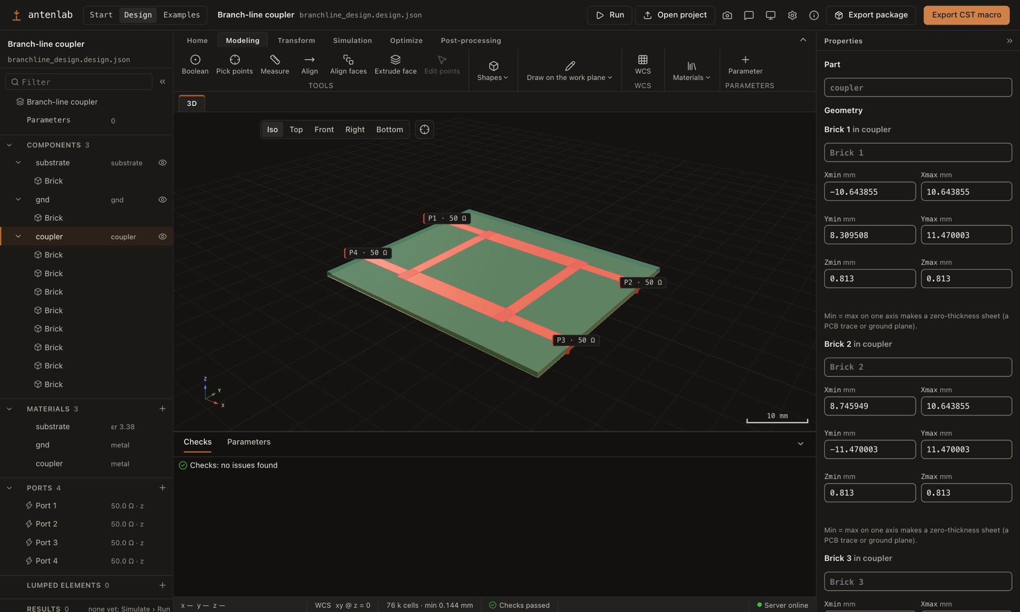
Ribbon: one row of seven tabs, Home, Modeling, Transform, View, Simulation, Optimize and Post-processing. The groups of a tab:
- Home:
- Project: Start, Import macro, Import PCB, Save, Close, Shortcuts.
- Edit: History (the modeling history), Undo, Redo, Duplicate, Delete.
- Modeling:
- Tools: Boolean (Add, Subtract, Intersect, Insert), Pick points, Measure, Align, Align faces, Extrude face, Edit points.
- Shapes: Brick, Cylinder, Sphere, Polygon, Extrude, Cone, Torus, Wire.
- Draw on the work plane: Brick, Circle, Polygon.
- WCS: Align with face, Transform WCS…, Align with global, Show WCS.
- Materials: Library, Add dielectric, Add metal.
- Parameters: Parameter.
- Transform: Transform… opens the transform dialog for the selected solid or shape. Rotate, Scale, Mirror and Translate copies open it with that operation selected. See Transforms.
- View: camera presets, Fit and Screenshot, followed by geometry/overlay visibility controls. Guide grid controls both the reference grid and active drawing-plane grid; it does not disable snapping. Ground plane controls only the model's PEC half-space geometry. Mesh view uses the same toggle as Simulation › Mesh. View preserves an active 3D result so its camera and overlays can be adjusted.
- Simulation:
- Frequency band, and while there is room the f min and f max fields.
- Boundaries.
- Mesh: the Cells / λ field (while there is room), Mesh settings, Mesh convergence…, Mesh view.
- Ports: Lumped, Waveguide, Add lumped element….
- Monitors: Far field, Surface current, Efficiency, Field plane.
- Solver: Solver limits.
- Run.
- Optimize: Parameter sweep, Optimizer.
- Post-processing: the result tabs to open (Summary, S-parameters, Smith, Efficiency, Pattern, 3D pattern, Currents, Field plane, Field map), Farfield (the pattern quantity, only while a pattern is shown), and Report and export (PDF report, Package, Python).
The ribbon remembers the last tab, except that a design with no parts opens on Modeling. Showing a result switches to Post-processing, and going back to geometry work returns to the tab you left. A double-click on a tab, the chevron at the right or Ctrl+F1 (⌃F1 on macOS) minimizes the ribbon. When the window is narrow, the buttons lose their labels (the tooltip keeps the name) and then whole groups fold into drop-down buttons, so every command stays reachable.
- Home:
Navigation tree (left): the design and its Parameters row (it opens the Parameters tab of the dock), then Components, Materials, Ports, Lumped elements and Results. A red or amber mark shows that a check points at that item. The simulation settings are not in the tree: they are the Simulation tab of the ribbon. See The navigation tree.
Main area: the 3D view is the first tab and never closes; the result views of a run (S-parameters, Impedance, VSWR, Smith, Efficiency, Pattern, Table) open as further tabs beside it. Ctrl+Tab and Ctrl+Shift+Tab switch tabs; Delete or a middle-click closes a result tab.
3D view: the geometry as the run server builds it from your unsaved changes, so what you see is what openEMS will mesh. The browser draws each edit at once; the server's version replaces it a moment later. Click a part to select it. View sets the camera (Iso, Top, Front, Right, Bottom, Back, Left) without changing zoom or the viewing center. Fit frames the model while preserving its current orientation. Number keys: 1 snaps to the nearest axis, 2 Bottom, 3 Back, 4 Left, 5 Front, 6 Right, 8 Top, 0 Iso. Use the numpad (also with Num Lock off) or the number row. Camera shortcuts work while 3D is visible, except inside fields, editors, menus, dialogs, or an active drawing tool. With the 3D view focused, arrows orbit (Shift pans), +/− zoom, and Space or F fits the model. Orbiting away from a preset clears its pressed state. The number-row aliases are provided for laptop keyboards.
Properties (right): the fields of the selected item.
Dock (bottom): Checks and Parameters, and for a run started here Run (its live progress), Runs (the design's runs side by side, with the parameters that differ) and Log. Drag its top edge to resize all tabs together, from 120 px to 70% of the center height. Focus the edge and use arrow keys (10 px, or 50 px with Shift); Home/End choose the limits. The height is remembered in local storage and overrides responsive defaults. Double-click resets it. The left and right panel edges also resize in Design and Results (180 px minimum, 35% of the workspace or 600 px maximum). Arrow keys resize; double-click resets. Remembered widths override responsive defaults while panel toggles still hide the panels (Ctrl+Shift+1, 2 and 3 fold the tree, the dock and the properties; ⌃⇧1, 2 and 3 on macOS).
Status bar, left to right:
- the cursor position in the 3D view (on a part, else on the ground plane);
- the work plane;
- the units, mm and GHz;
- the cell count and smallest cell of the preview mesh (a click toggles the mesh view);
- the check summary (a click shows the Checks tab);
- a run in progress (a click shows the Run tab);
- the preview time; while the design has errors, Preview paused: N errors (a click shows Checks), and Preview failed with a Retry button when the server itself could not build it;
- the run server state (a click looks for the server again; the bar also checks it every ten seconds).
Close in the Project group (or File › Close Design in the desktop app) releases the open design and returns to Start. With unsaved changes, choose Save, Don't save, or Cancel. A failed save leaves the design open and explains the problem. The saved design remains under Your designs so it can be opened again. Close does not cancel a running simulation.
In the desktop app, Ctrl/Cmd+W closes the project (or the window when no project is open). In a browser, use the Close button; Ctrl/Cmd+W remains the browser tab shortcut.
Shortcuts: Ctrl/Cmd+S saves, Ctrl/Cmd+Z undoes, Shift+Ctrl/Cmd+Z or Ctrl+Y redoes, Ctrl/Cmd+Enter runs, Delete removes the selection, Escape clears the selection (or stops drawing). Home › Shortcuts (or ? in the designer) lists them all.
The navigation tree
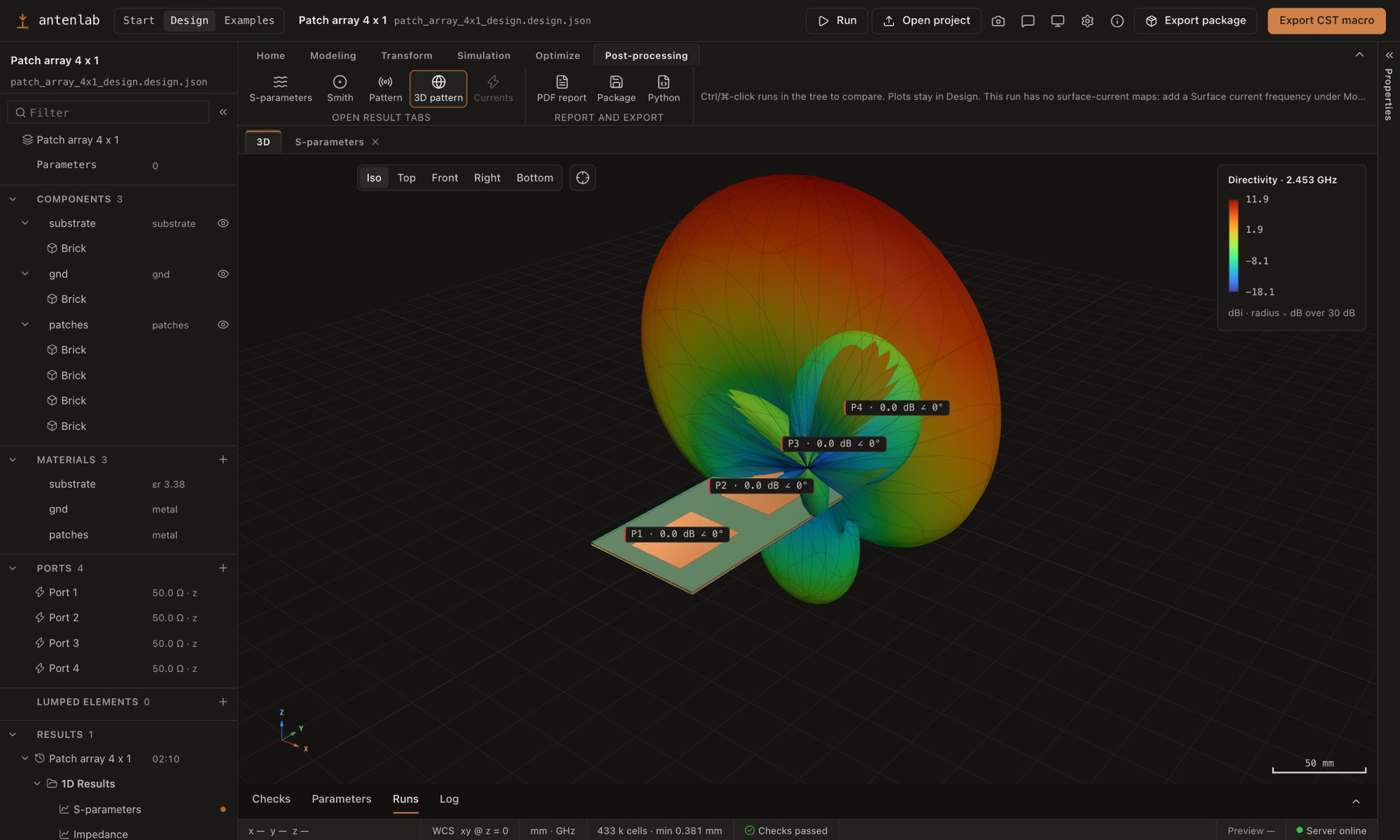
Parameters: one row with the number of parameters; a click opens the Parameters tab of the dock.
Components: the parts with their shapes, in component folders when they have one. Drag a part onto a folder (or onto the Components heading for the top level) to move it; right-click a part or shape for its menu.
Materials, Ports and Lumped elements (resistors); the + on a heading adds one.
Results: one node per run of the design, newest first, labeled with its name, time and engine. The newest is open. Under a run:
- 1D Results: S-parameters, impedance, VSWR, Smith chart, efficiency;
- Farfields: for each far-field frequency, the pattern cuts (Farfield (f = …)) and the 3D pattern (f = …);
- 2D/3D Results: one surface-current map per monitor frequency, and one node per E/H field-plane map, e.g. "E-field (z = 2.572 mm, 2.45 GHz)" (the mesh line the plane was recorded on, which may differ slightly from the position typed);
- Tables: the S-parameters and the impedance as numbers;
- Log.
The runs of a parametric sweep are in one Sweep … folder (right-click it for Compare all runs). The runs of a mesh convergence study are in one Mesh convergence folder, with the verdict in its detail line ("3 of 4 runs · converged at 30 cells/λ"); its first row, Convergence report, opens the report (Mesh convergence). A finished optimization is a node of its own with Optimization history, Open best, Save best as a run and Apply best parameters to design (Optimizer).
Selecting a result shows the run in the 3D view (the 3D pattern of a far field, the map of a surface current or field plane) or opens its plot as a tab in the main area. Selecting a geometry item, editing the design, choosing a ribbon tab other than Post-processing, or leaving the designer takes the pattern or map off the 3D view and goes back to the geometry; result tabs of the main area stay open. Ctrl/⌘-click further runs (or tick them under Compare in a result tab's toolbar, or click their labels in the dock's Runs tab) to compare up to eight, one color each: the result tab draws them together (S-parameters, impedance, VSWR, Smith, pattern cuts, table). For multi-port runs the S-parameter picker chooses the S_ij (dB or phase), drawn for every run in its color with one dash per picked pair, and the Smith chart shows the picked port of every run. The dock's Runs tab lists the design's runs by their short labels (A, B, …, the ones the legends use) with the parameters that differ between them marked and the solver time; a run's label there adds it to the comparison or removes it, its name shows it. Copy data (Ctrl/⌘+C) and CSV in the result tab's toolbar write what the plot shows: the picked S_ij in dB or phase, the Smith port, every compared run named like the legend; the format menu beside them chooses As plotted, dB, dB + phase, Re/Im, Linear magnitude + phase or All. The Figure menu beside them saves the plot as PNG (300 dpi) or SVG, with the design name, view and frequency as a title, always in the light style on white paper whatever the app theme. Figures, CSV and Touchstone files of a result share one name:
<design>_<view>_<frequency>_<run time>(for examplepatch_antenna_impedance_1.5-3GHz_2026-10-07T10-22-01+0300.csv), with the frequency of a sweep or of the selected far-field cut, the run time written without colons, and only letters, digits and_ . + -, so the name is valid on Windows and macOS. Touchstone files use the viewsparams.
The Filter box at the top keeps the items whose name or detail contains every word typed, with the folders above them; Escape clears it. The tree works from the keyboard: Up/Down move, Right opens or steps in, Left closes or goes to the parent, Home/End jump, Enter selects.
Modeling
Parameters and expressions
Every length (mm) and frequency (GHz) field takes a number or an expression over the parameters:
W/2, h + 0.035, wavelength(f0) / 4. The field shows the value as you type (= 16) and marks an
expression that does not evaluate.
- An independent parameter has a default value, a unit, an optional range and a label. Sweeps, the optimizer and the Run panel's form change it.
- A derived parameter has an expression over the parameters above it (for example
lam = wavelength(f0)). - Operators:
+ - * / // % **and parentheses. Constants:pi,c0,eps0,mu0. Functions:sqrt,sin,cos,tan,asin,acos,atan,atan2,exp,log,log10,abs,min,max,round,floor,ceil,radians,degreesandwavelength(f_GHz)(free-space wavelength in mm). The rules are Python's, and the run server's evaluator stays the authority. - Numbers are doubles (IEEE-754 binary64) on both sides: a number is read as the nearest double, as
JSON reads it, and every step of an expression is a double, so the browser and the server give the
same value (
9007199254740993 - 9007199254740992is0; Python's exact whole numbers are not used). A number, name or step that is not finite is an error, even when a later step would bring it back (1e999,1 / (1e308 * 10)).round(x, n)acceptsnwritten as2.0. Functions such assinorlogcome from each side's maths library and may differ in the last digit (about 1e-16). - Expressions use ASCII only: digits, letters,
_, operators, parentheses, commas and spaces. A whole number cannot start with0(07), and comments (#) are not allowed. - A parameter key is letters, digits and
_(ASCII), not starting with a digit, and not a function, a constant or a Python keyword (in,lambda,True, ...). Other names, such as__proto__,constructorormatch, are ordinary keys. The Parameters dock marks a refused key as you type. A design file that already has one does not load (the server's error names the key, as for any invalid design file) until the key is renamed in the file.
Add a parameter with ribbon Modeling › Parameters › Parameter or Add parameter in the Parameters dock:
it gets the first free key p1, p2, … and no unit (fill the unit cell for a length or a frequency; a ratio
or εr stays a bare number). Every keystroke in the table applies at once (the 3D view follows), except
in the Key cell: a new key applies on Enter or when the cell is left, and renames the parameter
everywhere it is used in one undo step (the shapes, transforms, cuts, ports, lumped elements, materials,
mesh and simulation fields, the other parameters, the operands a Boolean result keeps and the parameter
sweep), so renaming fw to feed_w leaves nothing that names fw. An invalid or taken key shows
its error under the cell and is not applied; Escape returns to the key as it was. A parameter that a
field still uses is not deleted (the trash button, Home › Edit › Delete, the Delete key): the message
names the places that use it, as for a material in use; Duplicate copies it as key_2.
Enter commits the cell and
moves down to the same cell of the next row; Escape takes back only what was typed since the
last commit, never a value already committed; leaving a cell (Tab, a click) commits it.
The compact table shows Key, Expression / value, Evaluated value, Unit and Description.
Min and Max are optional: Ranges reveals them, as does opening a sweep or optimization in the
Run panel. Existing limits stay in the file, and the run forms accept their own ranges.
Enter a plain number for a default or an expression for a derived parameter (marked =).
Descriptions edit in place; Label opens the optional display label. Validation remains on
fields and in Checks; focus or hover a cell to read its details. Arrow keys move between focused
rows, Enter edits the key, and Escape restores the cell's value before editing.
Unknown names in expression fields offer Create parameter inline after Enter or leaving the
field. The new value can itself be an expression of preceding parameters, such as lam/4.
Materials and parts
A material is a metal or a dielectric with εr, a loss tangent tan δ and the frequency where
tan δ holds (the band center if empty). Add one with ribbon Modeling › Materials › Dielectric or Metal.
A new dielectric (also one added from the library) gives tan δ at f0 when the design has an f0
parameter inside its band, else at the band center (the frequency left empty), not at a datasheet's
1 or 10 GHz.
openEMS applies tan δ as a constant conductivity, so the loss is exact at that frequency only and
scales as f_ref / f elsewhere: a datasheet value at 10 GHz used at 2.45 GHz gives four times the
loss. Give the frequency the design works at (e.g. f0); a check warns when it lies outside the
band. (A datasheet value taken at 10 GHz and used at 2.45 GHz made the patch starter's radiation
efficiency 65 % instead of 88 %; the starter now uses a value at its own frequency.)
A metal is a perfect conductor (PEC) unless it has a Conductivity (S/m; presets Copper 5.8e7,
Aluminum 3.5e7, Gold 4.1e7, PEC = empty) in Properties. A lossy metal's sheets become openEMS
conducting sheets (a surface-impedance model of a thin conductor, AddConductingSheet) of the
Sheet thickness (mm, 0.035 = 1 oz copper if empty; a thin brick built as a sheet keeps its drawn
thickness); its volumes become a material of that conductivity, which is only accurate where the
mesh resolves the skin depth (about 1.3 µm for copper at 2.45 GHz: never in an antenna mesh, so a
thick lossy volume behaves almost like PEC); wires stay perfect conductors. On the patch starter
(coarse, GPU) copper instead of PEC lowers the radiation efficiency at 2.45 GHz from 88.2 % to
86.5 % and the gain from 6.21 to 6.12 dBi. A macro's "Lossy metal" imports with its
conductivity, and the macro export writes one.
Modeling › Materials › Library lists common antenna materials with nominal values and their source: PEC (copper), FR4, Rogers RO4003C, RO4350B and RT/duroid 5880, Taconic TLY-5, alumina, PTFE and air. Add copies the values into the design as a new material, so the design file stays self-contained; edit the copy in Properties.
My materials. The library dialog has two groups, Built-in and My materials. Save a material of
the design to My materials with right-click in the tree › Save to my materials, or the button at the
bottom of its Properties: a dielectric keeps εr, tan δ and the frequency, a metal its conductivity and sheet
thickness, and both the color. Saving again under the same name updates that entry. Values that are
parameter expressions cannot be saved (the library holds plain numbers). Add on a My materials row
copies its values into the design like a built-in entry does, so a design file always carries a full copy of
every material it uses and its format does not change. The dielectrics of My materials are also offered as
the substrate of the PCB import. My materials… in the library dialog opens the list to rename, edit
(εr, tan δ, conductivity, thickness) and delete entries, Export it to a JSON file
({"version": 1, "materials": [...]}) and Import a file from a colleague: bad entries are skipped with a
warning, and a name already in use gets a number. The list is kept in materials.json in the workspace
when the run server is connected (see Run server and Run panel), else in this browser's
localStorage.
A part is one material and one or more shapes: in openEMS it is one CSXCAD property. Where parts overlap, the higher priority wins (metal 10, dielectric 0 by default; a shape can set its own). Select a part to rename it, change its material, put it in a component folder, add shapes, cuts or transforms.
Components. A part's Component field is a folder path such as antenna/feed; the tree groups
the parts in folders by it. The build ignores it (the exported Python names
it in a comment). A design without components loads unchanged: every part is at the top level.
To make a component, choose Move to component › on a part and type a new name (a / makes a
subfolder), or drag a part onto another part at the top level. Right-click a component folder for
Rename component (or F2 on the folder row; parts in its subfolders follow), Ungroup
component (its parts and subfolders move up one level) and Delete component and its parts;
Show parts and Hide parts act on everything inside. Each is one undo step.
Right-click a solid or shape in the tree or the 3D view for Rename, Hide, Transform…, Color…, Round corners… (on a box), Boolean ›, Move to component ›, Add discrete port here (when the picked metal face supports it), Duplicate and Delete. Rename edits the displayed label inline in the tree; a shape's label is saved in the design without changing its geometry. Move to component lists the existing folders in place (and a field for a new one). In the 3D view, Add discrete port here starts at the picked point and uses the face's dominant axis, offering the metals behind and in front of it (a patch's ground plane) as the other end. Review the endpoints before adding. Shift+F10 or the Menu key opens the menu for a focused tree item or the selected viewport part. Up/Down, Home/End navigate; Escape closes and returns focus. Blank viewport space keeps the browser menu.
Seeing what you add. A new shape, a drawn or extruded one, a duplicate, and a new port or resistor are selected and the 3D view fits them once, keeping your viewing direction: a port or resistor is framed with the smallest metal it touches, so you see where the feed sits. Selecting or editing afterwards never moves the camera; Fit (F or 0 in the 3D view) shows the whole model.
Shapes
The Modeling tab's Shapes group adds a shape:
- Brick, Cylinder, Sphere, Polygon and Extrude open a shape dialog with a shape of a sensible size on the work plane. Every value takes an expression, and the 3D view outlines the shape as you edit. Choose a new part (with its name and material) or an existing part to add it to. OK adds it in one undo step; Cancel adds nothing. The material starts as the dielectric while the design has no solid yet (the substrate is the first brick of a printed antenna), then as the material you used last for a new solid in this design, else the first metal.
- Cone, Torus and Wire add a new part with one shape in the design's metal; edit it in Properties.
Adding or duplicating a part or shape selects it and fits the 3D view to its bounds once, keeping the current viewing direction. You can immediately orbit, pan or zoom; subsequent edits and server previews leave the camera where you put it.
A part's properties also add more shapes to it. The kinds:
- Brick: Xmin/Xmax, Ymin/Ymax, Zmin/Zmax. Zero thickness on one axis makes a sheet (a patch, a ground plane, a trace).
- Cylinder: axis, center, radius, inner radius (above 0: a tube) and the range along the axis. With min = max the range has no length: a flat circle (a ring when there is an inner radius), a sheet. The build makes it a regular polygon with vertices on the circle, an even number of sides that keeps every edge within 0.01 mm of the arc and is never below 64 (a ring is two half rings, since CSXCAD polygons have no holes). The VBA macro exports a full circle as a Circle with a cover, a ring as polygons.
- Sphere: center and radius.
- Polygon: a flat sheet with corners in a plane (normal and elevation).
- Extrude: a polygon extruded by a length along its normal. In the shape dialog, a polygon with a height other than 0 becomes an extrusion.
- Cone: axis, center, the bottom and top radius (0: a sharp tip) and the range along the axis.
- Torus: axis, center, the major radius (axis to the tube center) and the minor radius (the tube). openEMS gets the tube as a 64-sided polygon turned about the axis.
- Wire: a thin wire along a polyline of points, with a radius. The automatic mesh puts fine cells around it.
- Polyhedron (
{"kind": "polyhedron", "vertices": [[x, y, z], ...], "faces": [[i, j, k, ...], ...]}): a closed solid from its vertices (expressions allowed, at least 4) and polygon faces (lists of vertex indices, at least 4 faces of at least 3 different, existing indices each). There is no drawing tool; it comes from an example (the pyramidal horn) or a JSON file, and Properties shows its vertex and face counts and the vertices read-only. The build (CSXCADAddPolyhedron) and the 3D view fan every face into triangles, oriented outward by the enclosed volume, so a mirrored copy still builds. Part transforms (move, rotate, scale, mirror, copies) map the vertices. The VBA macro format has no polyhedron, so the macro skips it and lists a warning; the Python export writesadd_polyhedron(...)with a small helper. The checks use its bounding box, and refuse bad indices (polyhedron) or vertices all in one plane (polyhedron-flat).
Drawing on the work plane
The Modeling tab's Draw on the work plane group draws with the mouse on the work plane in the 3D view:
- Brick: click two opposite corners.
- Circle: click the center, then a point on the rim (a cylinder, or a flat circle sheet when the height is 0).
- Polygon: click the corners; click the first point again, double-click or press Enter to close it.
A hint under the ribbon says what to click next and how many points are placed. Escape or Backspace removes the last point (the first one too, staying in the tool); Escape with no point placed stops drawing, and a tool armed again starts with no points. Enter before the first click opens the tool's shape dialog with default values. A finished shape opens the shape dialog, prefilled with what you drew, unless "Confirm drawn shapes in a dialog" is off in the group's Options panel; then it goes straight into a new part. Finishing a shape also leaves the drawing mode: OK in the dialog ends with the new shape selected and no tool left to cancel. A double-click or Enter finishes the shape, Escape cancels it.
Typed coordinates. While drawing, start typing (a digit, -, @, = or a letter) to enter a
point instead of clicking; Enter places it:
u, v: a point on the work plane; values can be expressions (W/2, L/2) and stay expressions in the shape.@du, dv: relative to the last point.- Brick, second corner:
w, his the size;=u, vgives the corner itself. - Circle, rim: one value is the radius.
Snapping. Points snap to the grid of the work plane and, when the pointer is close to one, to the corners, edge midpoints and edges of existing geometry on the plane (a dot marks the snap). The group's Options panel turns each kind on or off.
Work coordinate system (WCS)
The WCS is where drawing happens: the global WCS (u, v, w are x, y, z) is the starting point, and four buttons in Modeling › WCS change it:
- Align with face: click a face of a part in the 3D view. The WCS origin goes to the face centre and w along the face's outward normal (u along +x, or +y on a face looking along x). Only faces along x, y or z can be picked. The origin keeps the face's own expression: a WCS on "Substrate: top" sits at z = h and follows the substrate when h changes.
- Transform WCS…: one dialog. Move along u, v, w shifts the origin along the current WCS axes; Rotate about u, v, w turns the WCS (applied in that order, each about the axes the previous turn left), in multiples of 90° because the geometry stays axis aligned. Values take expressions (a rotation is evaluated to a number). The dialog shows the resulting origin and axes. With a point picked by Pick points, "Move the origin to the picked point" is offered too.
- Align with global puts everything back. Shapes already drawn stay where they are; points placed for an unfinished shape are dropped.
- Show WCS shows or hides the u, v, w arrows of a local WCS in the 3D view.
While a local WCS is active the corner axes gizmo, the 3D cursor readout, the status bar, the drawing readout, the typed-coordinate prompt and the shape dialogs say u, v, w instead of x, y, z, the work-plane grid is labelled u and v, and the status bar shows a Local WCS badge; clicking it (or Align with global) returns to the global WCS. With the global WCS everything is x, y, z.
Grid snap, the default height (the extrusion of a drawn brick or circle; 0 draws a sheet), what the pointer snaps to (corners, midpoints, edges), whether drawn shapes are confirmed in the shape dialog and "Look at the plane" are in the Options panel of the Draw group.
Shapes drawn or created from the Shapes palette in a local WCS are described in its coordinates: the dialogs show them, and the new part carries ordinary ordered rotate/move transforms that place it in global coordinates (parameter expressions stay expressions). Existing parts stay unchanged, and returning to global affects future drawing only. A face looking along -x, -y or -z gives a WCS whose w points the other way: the part then also carries a half-turn about an in-plane axis.
Saved with the design. A WCS other than the global one is stored in the design file as an
optional top-level wcs field (normal, origin as three expressions, angle in 90° steps, and
flip when w points along the negative axis), so it survives save and reopen. Designs without the
field open with the global WCS, the server ignores the field, and geometry never depends on it.
Every WCS change is one undo step. Unresolved or nonfinite origins are reported and cannot be
committed by the shape dialog or mouse drawing; correct them or their parameters first.
Transforms
Select a solid (or one of its shapes) and choose the Transform tab's Transform… button, the context menu's Transform… or Ctrl/Cmd+T (desktop app). One panel beside the 3D viewport holds the operations, chosen as Operation:
- Translate shifts the selection by an x, y, z step. With Copy off it moves the existing
geometry (each value accepts expressions); it is an ordered, editable transform, so a move after
an array moves the entire array in world coordinates, and a move before a mirror changes where the
mirrored result lands. With Copy on, the Repetition factor (copies to add) gives that many
more copies, the k-th shifted by k × step (the original stays). Values can be expressions, so
copies = N - 1andstep = [d, 0, 0]make an array that follows the parameters. Use last two picked points takes the step from two points picked with Pick points, and Pick anchor and place in viewport moves the part by clicking an anchor on it and a target. - Scale by x, y, z factors about an origin. Only positive, uniform factors are accepted.
- Rotate about x, y or z through a chosen center, by an angle in degrees. Positive angles follow the right-hand rule. Angles and center coordinates accept expressions. With Copy off (or zero copies) the original rotates; with a positive count the original stays and copies appear at angle, 2 × angle, and so on. Arbitrary angles are supported. Quarter turns retain the existing axis-remapping path; other angles attach a transformation matrix to the native primitive in CSXCAD. The solver uses the rotated shape, not its surrounding bounding box. Automatic meshing uses its world-coordinate bounds. Boolean operations on arbitrarily oriented operands remain unsupported and produce a validation error.
- Mirror across the plane through a Point on plane whose Plane normal axis is x, y or z; Keep original (add mirrored copy) decides whether the original stays.
Duplicate (Home › Edit, or Ctrl/Cmd+D) copies the selected solid, shape, port, lumped element, parameter or material; Delete removes the selection (a material or a parameter only while nothing uses it). A duplicated solid lies on its original on purpose, so it raises no overlap prompt; moving or editing it into another solid does.
Selection in the 3D view. The selected solid gets a red tint, an outline and an x-ray fill drawn over everything. When one shape of a solid is selected in the tree, only that shape gets the full highlight and the solid's other shapes a faint outline. Solids that enclose the selection (its centre lies inside them, such as a substrate around a via) are drawn faint while it is selected; solids that only touch it keep their look.
Transforms stay editable (and removable) in the part's properties; they are expanded exactly when
the model is built. Transforming one shape in a multi-shape part makes that shape an independent
part, retaining its material, cuts and earlier transforms, so its siblings stay in place. Ports and
lumped resistors do not move with the shapes: they stay at their world coordinates, and the panel
says so. When a transform leaves no original in place (a move, a rotation, scale or mirror without
the original kept) and ports sit on the selected metal, the panel warns prominently, names those
ports and offers Select port N for each: a port that no longer spans the gap between two
conductors gives |S11| of about 0 dB and no radiation (the checks flag it as port-floating, and the
run quality verdict as an uncoupled port).
The panel previews the result as an outline in the 3D view while you type. The viewport remains
interactive: orbit, zoom and change the camera without closing the controls. View rotation plane
looks along the selected axis to make planar rotations easier to inspect. On narrow layouts the controls sit below the view.
Preview refreshes that temporary outline; Apply commits it once, as one undo step, and closes the panel.
Cancel removes the outline without changing the design. Apply is available only when the preview
matches the current valid inputs. Switching operations resets the Copy choice to its default.
Editing the underlying design elsewhere closes the panel so an older preview cannot overwrite
the newer edit. A tilted polygon's local vertex coordinates remain editable in Properties, but
dragging those vertices on a world-aligned drawing plane is disabled.
Design and Python exports preserve arbitrary rotations, and the VBA macro exports them as Transform
steps after the shape (mirror, scale, rotate about x, y and z, translate; a shear as a matrix, with a
warning). Fabrication export supports boards rotated within
the XY plane; a tilted substrate is not flattened into an incorrect fabrication outline.
Zero-thickness metal sheets must remain parallel to a solver coordinate plane; lossy sheets must
also preserve their local normal axis under affine transforms. Rotating within their plane is
supported. To tilt metal out of that plane, model its finite thickness and resolve it with a suitable
mesh. These checks prevent a visible preview from implying unsupported thin-sheet solver behavior.
Right-click a component folder and choose Transform component to transform all its solids, including nested folders, around one shared origin/center/plane. The preview includes every member, and one Undo restores them all. Folder moves only change organization: drag the part row (or a single-shape part's shape row) onto a component folder. Move to component in the context menu provides the keyboard equivalent. Part material and geometry remain unchanged.
Booleans, picking and aligning
The Tools group (Modeling tab) holds the commands that work on several solids or on picked geometry:
Boolean combines two parts, A (kept) and B: Add (union), Subtract (A − B), Intersect and Insert (A − B with B kept). Select A, choose the operation (or press + − * / with A then B selected: the 3D view previews A op B, Enter or the same key again applies it). With A selected, the Tools › Boolean menu and the right-click › Boolean submenu list the other solids: Subtract › (or Add ›, Intersect ›, Insert ›) and one pick applies the Boolean at once, in one undo step. Without a selection, choose the operation, then pick B. The 3D view previews the result with the operands in color; Apply (Enter) keeps it, Swap A ↔ B exchanges the operands, Escape cancels. The result is live: it keeps its operands and is recomputed when parameters change, in the browser and in the build. It is exact for bricks, sheets and polygons whose planes share one normal (the exact clipping of bricks and polygons), and works for every other shape too, as listed below. Polygons along different axes, and the combinations marked refused, are refused with the reason. The Boolean menu's History lists the results.
Operation Bricks, sheets, polygons Cylinders, tubes, cones, spheres, tori, wires, polyhedra (alone or mixed with those) Add exact union exact: the shapes are kept together (A and B share material and priority, so overlap is a union); bricks and polygons are united Insert exact A − B exact: A stays whole, B (a part of its own) is lifted half a priority step above it Subtract exact A − B exact: B becomes a cut-out of A (a vacuum shape above it, see Cut-outs below). A cylinder minus a coaxial cylinder or tube is exactly a tube (a counterbore: tubes and cylinders) Intersect exact exact for coaxial cylinders and tubes, a tube or cone trimmed by a brick across its axis, a shape lying completely inside a brick, and cylinders with bricks or polygons along the cylinder's axis (the cylinder is clipped as a 64-gon prism; the native cylinder stays when the clip leaves its ring untouched, otherwise the clipped part is a 64-gon prism, within 0.12 % of the radius). Everything else (sphere ∩ cylinder, crossing cylinders, polyhedra, a sphere cut by a brick) is refused with the combination and what to do instead: Subtract the part you do not want (for example a brick on each side to cut away), or draw the common shape as an extruded polygon or a polyhedron Operands that already carry a cut-out (the result of a Subtract) can be subtracted from again (the cut-outs add up) or inserted, but not added to, intersected or subtracted: restore the operands from the History first. An overlap with curved shapes opens the same overlap prompt as for bricks (the shapes themselves are tested, not their bounding boxes). Arbitrary-angle rotations of the operands are refused for every shape, as before.
Pick points picks a Vertex, a Mesh midpoint or a Face / circle center in the 3D view; Measure shows the distance between two picked points and the included angle of the last three. A picked point can also fill a coordinate in the transform dialog and move the WCS origin.
Align picks a point on the part to move and then a target point. Align faces picks a flat face of the part and a target face: the part turns by quarter turns when needed and moves so the faces meet (Against, face to face) or lie in one plane (Flush), optionally centered on the target face. Only faces along x, y or z work (box and sheet faces, polygon and extrusion faces, the flat caps of cylinders and cones). The result is an ordinary transform.
Extrude face (key S) picks a flat face and asks for a Thickness, Material, Name and Component path; it adds a new part thickened from that face. The 3D view outlines the new solid (dashed, temporary) while you type the thickness.
Edit points lets you edit the corners of the selected polygon or wire in the 3D view: drag a point to move it, + inserts one, Delete removes one. Each change is one undo step.
Cut-outs (void carvers)
- Contract: any primitive may carry
"void": true; it lives in its part'sprimitiveslist, the part's transforms apply to it, the part's sheetcutsdo not. Older readers ignore the marker. - Build: a void becomes vacuum (eps_r 1, mu_r 1, lossless; a property named "<part> (cut)") with the priority given explicitly, or else the highest priority of the part's own solid shapes + 0.5 (default 10 for metal, 0 for dielectric), so it erases every lower-priority material inside it. Fractional priorities are ranked to integers (order and ties kept; ports and resistors keep their place at 5) only when a design has one.
- Warning: the check
boolean-cut-eraseswarns when another part with the same or a lower priority lies inside a cut-out (it is erased too);boolean-cut-reachwarns when a cut-out leaves a gap to a zero-thickness sheet of its own part, or has no thickness, and so removes nothing. - A Subtract with a curved shape (or one cut across a sheet) is stored this way: the result's
primitivesare A's shapes followed by B's asvoidshapes, with the history (operation, A, B) beside them. A cut-out only removes a zero-thickness sheet (a ground plane) it reaches: measured with openEMS 0.37 (PEC edge counts), a volume crossing the sheet and one whose face lies exactly on it cut it alike, one with a gap and a flat (zero-thickness) one cut nothing. A face within rounding of the sheet is therefore made to lie exactly on it, and a flat B is refused. The cut-out also erases everything of equal or lower priority inside it (a pin through a hole in the ground needs a priority above the ground, such as 11, and the substrate inside the hole is erased unless it has a higher priority): the check says so. - 3D view and exports: the cut-out is drawn as a dashed translucent ghost in the Subtract colour on top of the solid ("A with a hole"), in the Boolean preview too. The VBA macro export emits a real
Solid.Subtractof a vacuum tool solid from each host shape (andSolid.Insertfor an Insert by priority, from the designer); STL, GLB, Blender, fabrication and drawing exports skip cut-outs. The bundle marks the vacuum partvoid: true(docs/BUNDLE.md); other readers see an ordinary eps_r 1 part.
Cuts (boolean subtraction)
A part's properties have Add a cut, Add a round hole and Add a polygon cut: a shape removed from the part's flat sheets in the same plane, for slots, U-slots, E-shapes, inset notches and clearance holes. A rectangle cut is given like a sheet brick (min = max on the sheet's axis); a round hole by its plane (normal and position), center and radius, built as a regular polygon like a flat circle; a polygon cut by its plane and points. Values take expressions. Cuts apply before the part's transforms, to every flat sheet in their plane: rectangular sheets, polygons and flat circles. CSXCAD polygons cannot have holes, so the build replaces each cut sheet by the exact difference: boxes when only rectangles cut a rectangular sheet, otherwise polygons clipped in 2D (a hole leaves its surround as several polygons that meet along their edges).
What stays refused, with a check that says why: a cut does not remove volume. When the cut plane crosses a solid of the same part (a brick with thickness, an extrusion, a real cylinder, a sphere, ...), that shape is left whole and the cut-unsupported check says so; make the shape a sheet or carve it with a Boolean subtract. A live Boolean of bricks cannot take a round or polygon cut on an operand (the sheets would become polygons); use a rectangle cut or apply the cut before the Boolean.
Ports and resistors
Ribbon Simulation › Ports › Lumped or Waveguide adds a port; its properties switch it between Lumped and Waveguide.
- Lumped port: a number, an impedance, a start and stop point and the current direction (x, y or z). A probe feed runs from the ground plane to the patch: start and stop differ only along the direction.
- Waveguide port: a rectangular waveguide port (openEMS RectWGPort) with a TE mode (TE10 by default), the width a and height b of the guide across the propagation direction, and start and stop spanning the guide cross-section: the excitation in the start plane, the probes in the stop plane. The properties show the cut-off frequency of the mode, and "Fit the port box to a × b" sets stop from start. openEMS excites TE modes only. Run the guide into a PML boundary behind the port so the backward wave is absorbed.
- "Excited (driven) port" chooses whether a port is driven; with several driven ports, Fairbeam runs once per port and stores the S-matrix (Multi-port structures).
- Resistor (Simulation › Ports › Resistor): a lumped resistor between two points, for terminations and loads.
Grouped discrete ports (opt-in). In a lumped port's properties, Add grouped feed adds a physical feed while keeping one logical port number, excitation selection and reference impedance. Move the added feed before running; it initially copies the first feed and the overlap check blocks that duplicate gap. Choose Parallel or Series and the additional feed's polarity (+1 or −1); the first feed always has positive polarity. All coordinates support expressions. Removing the last additional feed returns to an ordinary port. Remove additional feeds before switching to a waveguide port.
For N feeds and logical resistance R, Parallel uses N·R per physical termination, averages signed voltages and sums signed currents. Series uses R/N per termination, sums signed voltages and averages signed currents. These operations select a mode; they do not add wires or join solids. For a differential pair with the same geometric orientation, choose Series and −1 on the second feed. Oppositely oriented ground-to-strip feeds may instead use Parallel with +1 on both. Source strengths account for each gap length, so member voltage strengths follow these signs.
Save/reopen, Python Apply/export, previews, mesh checks, drawings and fabrication feed locations
retain all members. The official Python entry point is
sim.lumped_port(..., group={"connection": "parallel", "members": [...]}); an optional integer
group.priority defaults to 5. Each member contains start, stop, direction and optional
polarity. There may be 1–15 additional feeds. Custom measurement adapters remain unsupported
by Python-to-Designer conversion. The Export dialog refuses a VBA macro with grouped electrical
ports; the package export writes a geometry-only macro instead (no ports or lumped elements, noted
in its header).
The reported impedance, S-parameters and accepted power belong to the selected mode. Orthogonal member modes are excluded, so modal power need not equal the sum of physical member powers in an unbalanced field. These format and normalization tests establish no mesh-converged result for Examples 7.7 or 7.8.
Designs use the automatic mesh; a hand-made mesh needs a Python model (Writing models).
Checks
The Checks list in the dock watches the design as you edit. Instant checks run in the browser: expressions and parameter ranges, inverted or flat bricks, radii and lengths of the other shapes, polygons, empty parts and duplicate names, cuts, the ports (length, overlap, impedance, the waveguide mode, size and cut-off), resistors, the materials and the band. The server adds its own with every preview: the design must build, the far-field and monitor frequencies must lie in the band, and the mesh is checked. Errors stop a run, warnings do not, and notes (ⓘ) only say what the build does that the drawing does not show.
The server's checks include the causes of runs that cannot converge or hardly radiate:
excitation-too-long: the excitation pulse (about 2 ns at f max = 3 GHz) takes more than half of the timestep limit, because a tiny cell makes the timestep tiny (a warning). At or above the limit the run cannot converge at all: that is an error, and the run is refused until the mesh or the limit changes.thin-metal(note): a metal brick far thinner than the mesh can resolve, such as 35 µm PCB copper, is built as a sheet (see Mesh under Simulation settings).port-in-metal: a lumped port that reaches into a metal volume, which shorts it. A port spans the gap between two conductors, from the face of one to the face of the other. Metal across the port's middle is an error (the run is refused); an end that only reaches into metal is a warning.port-at-null: a probe at the center of the plate it feeds. For a patch that is the voltage null of the TM10 and TM01 modes: the feed sees almost 0 Ω. Move it about 0.15 × the resonant length off the center.metal-overhang: a metal plate or sheet lying on a dielectric face (or inside a dielectric layer) that reaches past the dielectric's edge into the air, for example a patch wider than its substrate. The message says by how much and on which side ("by 1.2 mm (x+)"). Metal that runs onto another metal body past the edge (a connector) is not flagged, and neither is metal that lies on no dielectric at all, such as a horn or a wire antenna in the air.metal-floating: metal that touches no other metal, no dielectric, no port, no resistor and no PEC boundary, and that is plainly misplaced: it hovers just off the structure (within 5 % of its own size of a dielectric or of connected metal, such as a patch left above a substrate that got thinner), it lies in the plane of a dielectric face but off its edge, or it is a solid block in the air. Plates and strips further away (a director, a reflector, a stacked patch on an air gap) are taken as parasitic elements and not flagged.air-pad: an explicit air padding (Simulation settings › Mesh) under half of what the automatic one gives, a quarter wavelength at f min (an eighth without the far field), so that the open boundaries and the far-field box sit close to the structure. Zero (the structure runs into the boundary) and designs whose sides are all PEC or PMC are left alone.
One-click fixes. Where the fix is unambiguous, the check carries a button that edits the design in one undo step; it re-checks when it is applied, so the check goes away:
| Check | Button |
|---|---|
tan-d-band |
Give tan δ at f0 (the band center when the design has no f0 inside the band) |
port-in-metal (an end reaching into metal) |
Move the end onto the face of 'gnd': the metal's own face on the port's side |
port-floating |
Move the end onto the nearest metal face: a face of metal along the port's axis within half the port's length |
no-port (no port at all), port-floating |
Add a discrete port… opens the discrete-port dialog (the check's own button, beside the fix when there is one) |
no-port |
Add a probe port between 'gnd' and 'patch', only for exactly one patch over one ground plane and no other metal: from the ground's face to the patch's, 0.15 × the patch's shorter side off its center |
metal-overhang |
Trim the metal to 'substrate': clips a brick drawn as it is (no array, cuts or live Boolean) to what it lies on, unless that would cut it off a port |
air-pad |
Set the air padding to λ/4 (λ/8 without the far field) |
port-at-null, excitation-too-long |
move the feed off the center, raise max timesteps |
The fixes use the design's own expressions where they give the right value (a port end moved to
h, a patch trimmed to G/2), so the edited design stays parametric. Without an offer the check
is ambiguous: an array, several patches, a port in the middle of a metal body.
Both look at the resolved, transformed geometry through bounding boxes, which are exact for bricks, sheets and their quarter-turn rotated copies. Only bricks and polygons are judged; round and bent shapes only count as something that metal touches, so an approximate box can hide a problem but not invent one. They are skipped while the design has errors. Like the other geometry checks, clicking one selects and frames the part in 3D.
A run that stopped at the timestep limit says why in Results: either the excitation pulse took most of the limit (with the timestep and the smallest cell), or the fields decayed slowly.
Click a check (or press Enter or Space on it) to expand its explanation. Geometry checks also select and frame the item in 3D; focus stays on the check. Use Show in 3D to frame it again, or Edit field to focus the input. Non-geometry checks also require Edit field to jump to their field. The explanation stays open while its value changes and closes when the check is resolved. The dock's Checks tab shows the count, and so does the status bar.
Saving is always allowed: a work in progress with errors is fine on disk, and the save message counts the errors. The run server refuses to run a design with check errors (HTTP 422 with the list), whether the run comes from the designer, the Run panel, a sweep or the optimizer.
Simulation settings
The Simulation tab's buttons (Frequency band, Boundaries, Mesh settings, Far field, Surface current, Efficiency, Field plane and Solver limits) each open the Simulation settings dialog at their section: Frequency, Boundaries, Mesh, Monitors and Solver, listed on its left. The dialog edits the design at once (the preview follows, Undo reverts); OK keeps the changes and Cancel goes back to the design as it was when the dialog opened, with its undo history (once something was edited the button reads Discard changes). The Simulation tab also has the frequency and cells per wavelength fields inline, so the common values can be changed without the dialog.
Frequency (Frequency range): f min and f max of the excitation (GHz, expressions allowed). The mesh uses f max, the air around the model f min.
Boundaries: an unfolded box of the six faces (y− faces you, z+ on top). Click a face, then choose its type, or set all six at once:
- Open (MUR): an open, absorbing boundary (cheap); the patch starter and the empty project use it;
- Open (PML, 8 cells): an open boundary that absorbs better, with 8 extra cells; the other starters use it;
- Electric wall (PEC): for a ground plane or an electric symmetry plane;
- Magnetic wall (PMC): for a magnetic symmetry plane.
Open, add space is the air between the model and the open faces (
mesh.pad, mm; empty: a quarter wavelength at f min).Mesh: the Mesh mode is Automatic (recommended) (the adaptive mode: values appear as optional overrides, each with the value and reason the server chose), Classic (old) (shown only for a design that already uses its cells-per-wavelength, edge-rule, cell-ratio and air-density settings) or Manual lines (only for a design that has them, e.g. from an example; Switch to automatic mesh replaces them). This section also shows the preview mesh, the smallest cell and a solver-time estimate. The mesher is described in Automatic meshing. Mesh convergence… here (also in the ribbon's Mesh group) checks whether the mesh is fine enough (Mesh convergence), and Show the mesh view turns the mesh view on.
- Thin metal (
mesh.thin_metal): "Model as sheets" (the default) builds every metal brick thinner than a tenth of the finest target cell (λ at f max / cells per wavelength / √εr of the densest dielectric) as a zero-thickness PEC sheet. The sheet goes on the face that meets the substrate (else the middle), and port and resistor ends inside the copper move onto it. Draw copper with its real thickness: the display and the exports keep it, only the mesh ignores it. At 2.45 GHz the skin depth of copper is about 1.3 µm, so 17–70 µm changes the fields very little, but meshing it would make the timestep about 30 times smaller. "Mesh the thickness" keeps the volume only of plates at least 0.6 of the finest cell thick; thinner plates (35 µm copper) stay sheets there too, because cells across them make the timestep 30 to 60 times smaller and the run last 5 to 25 minutes or never converge.
- Thin metal (
Monitors:
- Far field (on or off) and its frequencies (empty: the |S11| minimum of each matched band), and an
optional Set phase center (mm). A design file can also set
far_field.faces, six true/false flags (x−, x+, y−, y+, z−, z+) for the faces of the near-to-far-field box that record; a face a feed waveguide crosses is left out, as in the pyramidal horn example. There is no dialog field for it yet. - Surface current: frequencies at which surface-current maps are recorded on the metal
sheets, as
fairbeam run --fieldsdoes. After a run they are under the run's 2D/3D Results in the navigation tree. Ribbon Simulation › Monitors › Surface current opens this field; when the design has none yet it starts with the far-field frequencies (else the band center), which Cancel takes back. Far field next to it opens the far-field settings. - Efficiency over the band (off by default): the radiation efficiency at N frequencies
(default 21, a whole number from 3 to 201) evenly spaced across the band, stored as
monitors.efficiency: {"points": N}and in the bundle'sresults.efficiency; total efficiency follows with the port's S11. It is computed from the far-field box after the run, so it adds post-processing time, and it needs the far field: with the far field off, or a count outside 3–201, themonitor-efficiencycheck (browser and server) is an error that blocks the run. Ribbon Simulation › Monitors › Efficiency turns it on (Cancel takes it back) and opens its Number of frequencies field. - Field planes: up to 4 cut planes, each recording the E- or H-field magnitude (|E|, or one
component |Ex|, |Ey|, |Ez|; the same for H) at 1 to 4 frequencies inside the band. A row sets
the quantity, the plane normal (x, y or z), the position along it in mm (an expression, e.g.
h + 1) and the frequencies; Add field plane and Remove edit the list. Stored asmonitors.field_planes: [{"quantity": "E", "normal": "z", "position": "h + 1", "frequencies": ["f0"]}]("component": "x"for one component). openEMS records a frequency-domain E or H dump on the mesh line nearest the position, across the whole domain; the values are peak phasor amplitudes in V/m or A/m for 1 W incident power at the driven port (one excitation, as for the surface currents). Thefield-planecheck (browser and server) flags more than 4 planes, a plane without a frequency or with more than 4, and a frequency outside the band;field-plane-position(server, it needs the domain of the preview) a position outside the simulation domain. All are errors that block the run. Ribbon Simulation › Monitors › Field plane adds a plane when there is none (E, normal z, 1 mm above the top of the model, at the far-field frequencies, else the band center; Cancel takes it back) and opens its position.
- Far field (on or off) and its frequencies (empty: the |S11| minimum of each matched band), and an
optional Set phase center (mm). A design file can also set
Solver: the end criterion (the field-energy decay that stops the run: −40 dB is quick, −60 dB accurate) and the timestep limit. The end criterion is a number from −10 to −300 dB: the field, the
end-criterioncheck (browser and server) and the run use these bounds, and a value outside them (−5 dB, say) is an error that blocks the run. −10 dB is Fairbeam's limit for usable results (above it the fields have barely decayed), not a physical one; −300 dB is the lowest a run accepts. Max. timesteps left empty ("auto") is chosen from the mesh: at least 60,000, the excitation pulse and its decay, or what about 1e11 cell-steps allow (up to 600,000), whichever is most; a run that converges stops earlier anyway. A thin low-loss substrate (RT5880 at 0.254 mm rings for ~50 ns, ~280,000 timesteps) needs that room; theslow-ringdowncheck warns when an explicit limit is below the estimated ring-down.
Mesh view
Ribbon Simulation › Mesh view (or a click on the cell count in the status bar) shows the FDTD mesh lines of the current preview on one plane and fades the solids so the lines show through. The mesh comes from the same mesher the run uses. The panel over the 3D view has:
- the plane controls: x/y/z and a slider through the mesh lines;
- the lines per axis, the cell count, the smallest and largest cell, and the timestep;
- a solver-time estimate.
The estimate is cells × timesteps divided by a conservative throughput from Benchmarks: the M5 Pro CPU engine with 4 threads measured 318–329 MCells/s and 250 is assumed, less for small grids. The GPU engine assumes 700 MCells/s. The timesteps are 15 to 80 periods of the band center. How long a run really takes depends on how fast the field energy decays, which is known only afterwards, so treat the range as a rough guide.
Mesh convergence
Ribbon Simulation › Mesh › Mesh convergence… (or the same button in Simulation settings › Mesh) checks whether the mesh is fine enough. The design runs at increasing automatic-mesh densities (cells per wavelength at f max), and each run is compared with the previous one:
- the resonance frequency (the S11 minimum of the first matched band, else the global minimum);
- |S11| at the resonance (dB);
- Dmax at the far-field frequency closest to the resonance (only with the far field on);
- the input impedance at the resonance (shown, not part of the stopping rule).
The dialog sets:
| Field | Default | Meaning |
|---|---|---|
| Densities | 15, 20, 30, 40 | Cells per wavelength, coarse to fine |
| Resonance change below | 0.5 % | Tolerance of the resonance frequency |
| |S11| change below | 1 dB | Tolerance of |S11| at the resonance |
| Dmax change below | 0.2 dB | Tolerance of Dmax |
| Run limit | 4 | The study runs at most this many densities from the list (a note appears when the list is longer) |
| Engine | the Run settings | CPU or GPU, when the server has both |
The study stops at the first step whose changes are all strictly below their tolerances. It then reports converged at N cells/λ, where N is the coarser density of that step: the finer run confirms it. When the densities or the run limit are used up first, it reports Not converged and names the quantity that was still moving, for example "resonance still moves 0.8 % between 30 and 40 cells/λ (limit 0.5 %)", and advises a finer density or a look at the model. A failed or stopped run ends the study too. In the results table the Within tolerance column says, for each run, whether its change from the previous run is inside every tolerance.
Before anything runs, the dialog builds a geometry preview at every density (nothing is simulated) and shows the mesh cells and a solver-time estimate per density, and the total if every run is needed. Above 10 minutes it warns and the button reads Start anyway. The estimate is the one of the Mesh view.
Start saves the design (check errors block it, as for a run) and queues the first density. The
next density is queued only when the previous run is done and the rule says to continue, so a
study that converges early costs no more runs. The dialog then shows the progress (with Stop)
and, as the runs finish, the report: a table of every quantity and its change per density, small
plots of the resonance, |S11| and Dmax against the density (the converged density filled), and
the verdict. Apply N cells/λ to the design sets that density (mesh.cells_per_wavelength, or
the cells_per_wavelength override in the Auto mesh mode); Undo takes it back.
The study works with both automatic modes (Automatic (recommended) and Classic (old)). An air density set by
hand is scaled with the density. A design with manual mesh lines cannot run a study: switch to the
automatic mesh first. The runs are normal runs of the design (one bundle each, named
<design>--mesh-<density>), so every result view and the comparison work on them. The server
keeps the study in studies/<id>.json next to the bundles (Sweeps and studies); the same
study runs from the command line with fairbeam converge <design>.design.json.
Running and results
Run (Simulation tab, the Run button in the header, or Ctrl/Cmd+Enter) opens the Run the simulation dialog:
- Engine: CPU (multi-threaded), or GPU (Metal or CUDA build) when the server has that build (GPU engine).
- Threads for the CPU engine (4 is a good default).
- S-parameter sample points: the S-parameter samples over the band (801 by default, 11 to 20001).
- Result name: leave blank to keep a unique bundle for every run (model id plus run suffix). A run never replaces an earlier one: a name that is already taken gets a short id added.
The dialog also shows the solver-time estimate (with one run per excited port when there are several). Its Run button (Save and run when there are unsaved changes) saves first. It refuses while the Checks list has errors: the dialog lists them, and a click goes to the field. A check that knows the fix offers a button, here as in the Checks list (see below): for example, when the excitation pulse alone needs more timesteps than the limit, Set max timesteps to N raises the limit (times are shown as 1.18 ps, not 1.18e+03 fs). While the run is blocked the dialog shows no time estimate. Optimize… opens the optimizer instead.
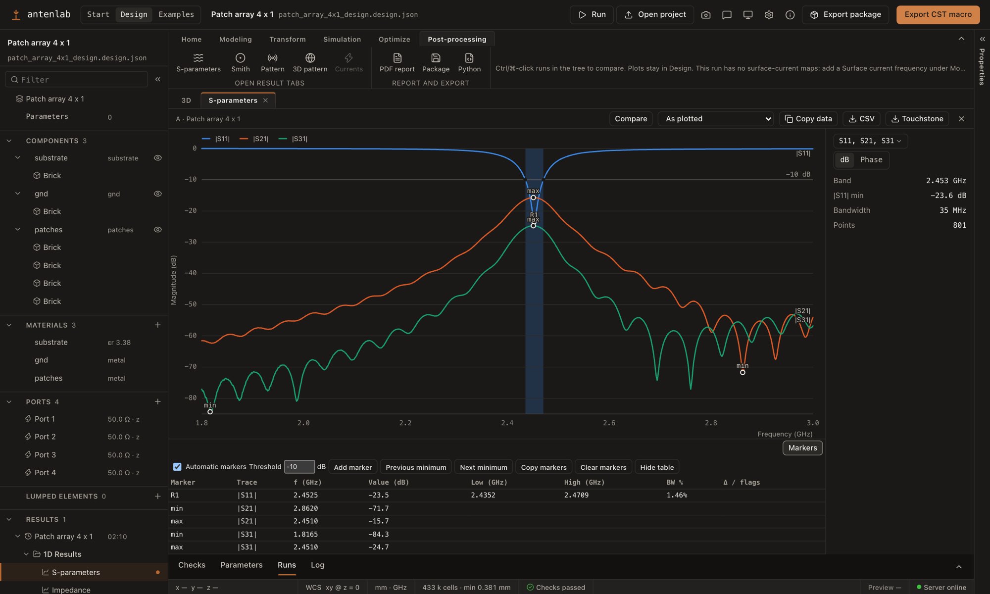
The run's progress appears in the dock's Run tab (and as "Running N %" in the status bar):
- the phases;
- the timestep, the speed, the field energy against the end criterion, the elapsed time and an estimate of the time remaining;
- a convergence chart;
- a Cancel button.
The 3D view keeps showing the design, and you can go on editing (the run uses the saved file).
Run quality. Every finished run gets a verdict (src/lib/runQuality.ts): converged, not
converged (it stopped at the timestep limit, so S11 and the far field may be wrong) or suspicious
(|S11| above 0 dB, a radiation efficiency above 100 %, or a port that is not coupled: |S11| of
-0.5 dB or higher over the whole band and/or a total efficiency under 2 % in every far-field entry,
typically a feed that no longer spans a gap after the geometry was rotated). "Converged" only means
the field energy reached the end criterion; it says nothing about the match. A run that is not clean shows an amber
banner over its result tabs and in the Run tab, with the reason and what to change (raise max
timesteps or relax the end criterion; refine the mesh, move the boundaries away or lower the end
criterion; see the efficiency note), and a warning badge in the navigation tree and the Runs table.
When a run finishes without converging, the dock stays on its Run tab.
When the run finishes, it appears under Results in the navigation tree (runs finished in the Run panel too). Its result views open as tabs beside the 3D view, from the tree's result nodes or the Post-processing tab; the dock's Runs tab lists the design's runs and Log holds the openEMS output. Each run row in the tree carries its headline numbers (resonance, |S11| minimum and Dmax) under its name, and the Runs table has columns for the resonance, |S11| minimum, −10 dB bandwidth, Dmax and total efficiency (from the run's bundle; a run not read yet shows the frequency of its band's |S11| minimum from the project index):
- Summary (tree: Tables › Summary, or Post-processing › Summary): the run card. The converged banner (a run that is not clean shows the quality banner above it), the headline numbers (resonance, |S11| minimum, −10 dB bandwidth, Dmax, realized gain and total efficiency at the far field nearest the resonance), the matched bands, the far-field values, and what the solver did. With several runs selected it is a table with one row per run and a column for each parameter that differs between them; each run's difference from the Reference run is shown under (or, in the Δ view, over) the value. The reference is the oldest selected run by default (run A when it is selected) and can be chosen above the table; Copy data and CSV write the same table (English headers, decimal points) with Δ columns against that run and its name in the last one. A run whose |S11| minimum is at the edge of the band with nothing below −10 dB has no resonance: Summary, the Runs table, the tree and Properties say "no resonance in band (minimum at the band edge)", and a mesh convergence study of such runs reports its steps as not comparable instead of converged.
- S-parameters: |S11| with the −10 dB bands, or the driven column of the S-matrix for several ports. The side panel lists each matched band: its best match (the frequency of the |S11| minimum), the minimum |S11|, its center (the middle of the band edges), its range and its bandwidth. A band that continues past the simulated range is marked ≤ / ≥ at its open edge, and its width is a lower bound.
- Impedance, VSWR and Smith: the input impedance, the VSWR (2:1 marked) and the reflection on a Smith chart.
- Efficiency: the mismatch efficiency 1 − |S11|² over the band (% or dB), with the radiation
efficiency and the total efficiency (radiation × mismatch) as points at the far-field frequencies;
one color per quantity, or per driven port for multi-port runs. The radiation efficiency is only
known where openEMS computed a far field (add frequencies under Simulation › Monitors › Far
field); a run that stores it over the band (
results.efficiency) draws it, and the total efficiency, as curves. Values above 100 % are unphysical and flagged. Where the port accepts only a few % of the incident power, the efficiency depends on how far the ring-down had decayed when the run stopped; values whose accepted power is uncertain by more than 10 % are left out of the curves and drawn as flagged points, with a note (a lower end criterion, e.g. −70 dB, makes more of the band reliable; Project bundle format has the measurements). - Pattern (with a far field): the φ = 0° and φ = 90° cuts of the chosen quantity with Dmax, gain, realized gain, radiation and total efficiency and the main-lobe direction; one chip per far-field frequency. Show in 3D in the tab's toolbar draws the same far field as a 3D pattern in the 3D view.
- Surface current (with a monitor): a tree node per frequency, or Post-processing › Currents; the map itself is drawn in the 3D view.
- Field plane (with field planes): each map has two nodes under 2D/3D Results, … · 2D map and … · 3D. The 3D node (or the ribbon's Post-processing › Field plane, the run's first map) draws the map in the 3D view as one semi-transparent heat-map plane at its true position. The color bar at the top right names the map and the driven port, and switches between dB (0 dB = the map's maximum, 40 dB range) and Linear (0 to the maximum, in V/m or A/m). Maps are recorded in the run; changing the planes needs a new run.
- Field map (with field planes): the 2D map node, or Post-processing › Field map, opens
the same map as a heat map in a main-area tab: axes in mm at one scale, the color bar with
dB / Linear, the projection of the model's parts onto the plane as an outline (solid for
metal, dashed for dielectrics; Structure outline turns it off), and a readout of the value
under the pointer (or, with the map focused, under the arrow keys; Shift moves ten samples,
Escape clears it). A Map picker switches between the run's maps and Show in 3D draws the
map in the 3D view. Copy data and CSV give one row per sample: u and v in mm, the magnitude,
and (with phase data) the real part, imaginary part and phase in degrees of each stored
component; English headers, decimal points. Runs made before phase data existed show the
magnitude only, with a note.
- Phase and Animate (the 2D tab and the 3D color bar share them): Phase colors the phase of one component against the incident wave of the driven port (a cyclic color scale, gray where the field is too weak to have a phase; for a map of |E| the strongest component, or pick Ex, Ey or Ez under Component). Animate shows the instantaneous field Re{F·e^(jωt)} over one period: a component as a signed value (blue-light-red), a map of |E| as the instantaneous magnitude |E(t)|. Play steps the period in 24 frames (one second per cycle) and pauses when the page is hidden or the system asks for reduced motion (the slider still steps through it); the 3D view redraws the same plane at each instant. The dB / Linear scale applies to magnitudes only.
- Examples: in the Examples viewer, a bundle with field planes lists them under Field plane in the model panel; the chosen map is drawn in the 3D view with the same color bar, phase and animation.
- Table: frequency, |S11|, VSWR and the impedance.
- Log (dock): the openEMS output (the end of it for an earlier run), with a link to the full log.
The far-field quantity (Directivity, Gain, Realized gain, and RHCP/LHCP directivity when the
run has circular-polarisation data) is chosen in the Pattern tab's side panel, in the far-field card
of the 3D view, or under Post-processing › Farfield › Quantity while a pattern is shown; the
choice holds for the session. Gain is the directivity plus 10·log10(η_rad), realized gain the directivity plus
10·log10(η_rad·(1 − |S11(f)|²)) with the driven port's S11 at the far-field frequency, so their
maxima are the bundle's gain_dbi and realized_gain_dbi. Without a radiation efficiency the
gain options are disabled (the tooltip says why) and the pattern stays directivity.
While the 3D pattern is shown, a card at the top right of the 3D view holds its color scale, the quantity, the far-field frequency chips (and driven port for multi-port runs), Dmax, gain, realized gain, radiation, mismatch and total efficiency and the main-lobe direction θ, φ. Its chevron folds it to the color scale alone. A multi-port array shows the array pattern (all ports fed), which has directivity only.
Another run opens from the tree. The header's exports (Export package, Export VBA macro) and Post-processing › PDF report / Package take the run shown. The ✕ at the right end of a result tab's toolbar closes the shown run (its result tabs and the dock's Runs and Log tabs); the ✕ on a tab closes that tab only. Each tab's toolbar also has Compare, the data-format menu, Copy data, CSV and Touchstone.
Working with more than one project
The editor currently has one active design. Save it before opening another design from Start; each file keeps its own saved geometry and result associations, but reopening starts a new Undo/Redo history. The result tabs are views of the selected run, not independent project editors.
In a result tab, Compare groups the current design's runs separately from other projects. Select another project's saved result to overlay it without replacing the active design or its primary result. Up to eight runs can be compared. Project and run labels distinguish the curves and exported data. Results load only when selected; failed loads offer Retry or Remove, and figure capture waits until the selected comparison is ready. Switching designs clears the comparison. Independent editable project tabs and side-by-side project windows are not yet implemented.
The standalone Results viewer also compares indexed results through its Compare control. Submitted simulations continue on the server while another project is viewed; the queue runs one solver at a time. New designer runs, sweeps, optimization and mesh-convergence studies use a checked copy of the saved design captured at submission. Later edits do not change that queued input. Python models and older jobs still use their original paths; keep those sources unchanged while queued. See admitted design inputs (opens in a new tab) for exact scope. The multiple-project plan (opens in a new tab) records the state, window and session work still required for independent editors.
Sweeps and the optimizer start from the Optimize tab (Parameter sweep, Optimizer) and their runs appear under Results in the tree. Python models use the Run panel instead (Run server and Run panel, Optimizer), where a design also shows up under its name like any model.
A new sweep axis starts as the parameter's current value ±10 % in 5 steps (never its whole range), and picks a geometric parameter, not the design frequency; choosing another parameter re-seeds the range. The optimizer's first parameter is also a geometric one, with bounds of the current value ±20 %.
The optimizer checks every candidate of a design before it simulates it. A candidate with check
errors, or one whose values make metal overhang its substrate or float in the air
(metal-overhang, metal-floating that the design at its own values does not have), is not
simulated: the evaluations table lists it as Skipped with the reason (for example
"'patch' overhangs 'substrate' by 1.2 mm (x+)"), it costs at least the failed-evaluation penalty,
and the search goes on. Sweeps run every point as it is.
Files
Where: designs are saved in the run server's models folder, next to the Python models. Repository checkout:
python/models/. Desktop app:models/in the workspace,~/Documents/Fairbeamon macOS and%USERPROFILE%\Documents\Fairbeamon Windows.Saving: every save keeps the previous version in
model-history/. If the file changed on disk since it was opened, the designer says so; saving again overwrites it with your version.Format:
fairbeam.design/1, one JSON object, documented at the top ofpython/fairbeam/design.py(all shape kinds, waveguide ports, transforms, cuts and components). A complete, valid example, a probe-fed patch:{ "schema": "fairbeam.design/1", "model": {"id": "my-patch", "name": "My patch"}, "params": [ {"key": "f0", "default": 2.45, "unit": "GHz"}, {"key": "W", "default": 32, "unit": "mm"}, {"key": "L", "default": 40, "unit": "mm"}, {"key": "h", "default": 1.524, "unit": "mm"}, {"key": "lam", "expr": "wavelength(f0)", "unit": "mm"}, {"key": "G", "expr": "L + lam / 2", "unit": "mm"} ], "simulation": {"f_min": "f0 * 0.6", "f_max": "f0 * 1.3", "boundaries": "MUR", "end_criteria_db": -60}, "materials": [ {"name": "copper", "kind": "metal"}, {"name": "substrate", "kind": "dielectric", "eps_r": 3.38, "tan_d": 0.0027, "tan_d_freq": "f0"} ], "parts": [ {"name": "substrate", "material": "substrate", "primitives": [{"kind": "box", "start": ["-G/2", "-G/2", 0], "stop": ["G/2", "G/2", "h"]}]}, {"name": "gnd", "material": "copper", "primitives": [{"kind": "box", "start": ["-G/2", "-G/2", 0], "stop": ["G/2", "G/2", 0]}]}, {"name": "patch", "material": "copper", "primitives": [{"kind": "box", "start": ["-W/2", "-L/2", "h"], "stop": ["W/2", "L/2", "h"]}]} ], "ports": [{"type": "lumped", "number": 1, "R": 50, "start": [-6, 0, 0], "stop": [-6, 0, "h"], "direction": "z"}], "resistors": [], "mesh": {"mode": "auto", "cells_per_wavelength": 20}, "far_field": {"enabled": true, "frequencies": ["f0"]}, "monitors": {"currents": ["f0"]} }f0,W,Landhare independent parameters;lamandGare derived (a derived parameter may use the ones above it).monitorsis optional.monitors.currentsmakesfairbeam runrecord surface currents at those frequencies without a--fieldsflag;monitors.efficiency: {"points": 21}adds the efficiency over the band, as--efficiency 21;monitors.field_planesrecords E/H maps on cut planes, as--field-plane.Example designs: examples/designs/ holds designs to copy into your models folder, all for UAV telemetry at 867 MHz: a swept blade antenna, a slotted wideband planar dipole, a printed meander dipole for airframes without a metal skin, a printed sleeve dipole, a printed 2-element collinear and a ground-station 5-element Yagi, each with its results and how to scale it to other bands. The desktop app installs them in the workspace's models folder, read-only, as the sources of the 867 MHz examples: Open as new design… on one of them makes an editable copy. Their IDs, like those of the bundled Python models, are reserved for them.
Copies of examples: a copy of a bundled Python example keeps the example's description, the names and labels of its solids and the names of its materials. What the conversion did (the parameters it carried over, the ones it fixed) is in
model.conversion, shown as Conversion notes in the design's Properties.Command line: a design runs like a model file:
fairbeam run python/models/my_patch.design.json --set W=30(CLI reference).Python export: ribbon Post-processing › Report and export › Python (also File › Export › Python… in the desktop app) opens the Python source panel in place of Properties: the design as an equivalent Python model file (
MODEL,PARAMS,build), for hand editing or for features that designs do not have yet (Writing models). Copy puts it on the clipboard, Save… writes the.pyfile, and Refresh source appears when design edits have made it out of date. It builds the same geometry and mesh.Edit and Apply: Edit in the Python panel turns the script into an editor (line numbers, Python highlighting, Tab indents). Apply (or Ctrl/Cmd+Enter) sends it to the run server, which builds the geometry without running the solver and replaces the design's solids, materials, ports, parameters, mesh, simulation and far field with the result, in one undo step. The design keeps its name and id. The script is read back with the same converter as the bundled Python examples, so its rules apply: exact primitives only, coordinates that are linear in the parameters become expressions, the other numbers stay numbers, and a parameter that drives nothing is dropped. After Apply the panel writes the script again from the new design; when that script builds the same design your text stays, otherwise it is replaced and the panel says the script was normalized. A failure (a Python exception, a syntax error, an unsupported feature, a time-out) comes back with its line: the editor marks the line, the message shows under the header and the design is not touched. Done with changes that were not applied asks before discarding them. Edit needs a connected run server, because it runs your Python on your computer: the web demo shows the button disabled with the reason. The script runs in a child process with a 20 s limit and a 512 KB size limit, one at a time, and
FDTD.Run/Simulation.runraise instead of starting the solver. This is not a sandbox: the script can do whatever Python can, so apply only your own code.
Importing a VBA macro
Import VBA macro… (Start screen, Home › Project › Import macro, File › Import VBA macro…) reads a
CST-compatible VBA macro (.bas, .mcs) or a history list saved as text and shows the import
report before anything is saved: what was created, and every command that was not imported or was
changed on the way, with its line. Name the design and Create and open saves it and opens it
here. The command line does the same: fairbeam import-cst model.bas --out my.design.json.
What is read (python/fairbeam/cst_import.py, SUPPORTED): units; parameters (StoreParameter,
MakeSureParameterExists, ...) as design parameters, a value as an independent one and an
expression as a derived one (VBA ^, Sqr, Atn, Mod, \, Pi, clight, ... translated, and the degree
functions Sind, Cosd, Tand, Asind, Acosd and Atnd, whose angles and results are in degrees);
materials (Normal: εr and tan δ, a conductivity as the equivalent tan δ; PEC; lossy metals as PEC,
with a note); bricks, cylinders and tubes, cones, spheres, tori, polygons and rectangles or circles
covered or extruded, point-list extrusions; Solid.ThickenSheetAdvanced on a planar sheet (Inside,
Outside or Centered, taken relative to the sheet's face normal); a straight Loft (zero tangency) between two
convex, parallel sheets of the same outline, as a polyhedron; components; Solid.Add (a union), Solid.Subtract,
Intersect and Insert as live Booleans where the designer's Booleans can hold them (bricks,
sheets, polygons); transforms (translate, rotations by any angle, mirror, uniform scale, with copies);
axis-aligned local working coordinate systems; the frequency range, boundaries, the mesh density
(lines per wavelength), discrete ports, resistors, waveguide ports with given ranges, far-field and
H-field monitors. Coordinates are converted to mm and rounded to 1e-6 mm, the precision of the
mesh lines, so ports sit on mesh lines. VBA code itself (variables, If, For) is not run.
No shape is dropped silently: every object or operation that cannot be imported is named in the report
(for example a Loft with tangency or non-matching profiles). A loft that cannot be imported keeps its
profile sheets, and the dialog warns that the geometry is incomplete, so rebuild the connecting solid
before simulating.
Mesh density is read from Mesh.LinesPerWavelength and from MeshSettings blocks explicitly
marked SetMeshType "Hex" or "HexTLM". In those blocks, StepsPerWaveNear sets cells per
wavelength and StepsPerWaveFar sets air cells per wavelength only when positive and lower than
the near density. Tetrahedral, surface, unknown and unspecified mesh types do not set FDTD density:
their steps per wavelength are ignored. Without a supported density, Fairbeam uses its automatic
mesh default of 20 cells per wavelength. A supported hexahedral density is retained even if an
unsupported block appears later in the VBA macro. The import report explains the mapping or the
ignored density settings; review the mesh and design checks before running a simulation.
A macro exported by Fairbeam carries comments starting with fairbeam-data: with the exact
openEMS port boxes, the boundary types and the automatic mesh settings (other readers ignore them), so
exporting a design and importing the macro gives the same model back
(python/tests/test_cst_import.py). They are used only where they agree with the macro commands next
to them.
Importing PCB artwork (DXF/Gerber)
fairbeam import-pcb, and the Import PCB artwork… dialog (below), turn the 2D artwork of a
printed antenna into a design (python/fairbeam/pcb_import.py). It reads ASCII DXF (closed polylines, CIRCLE, ARC,
ELLIPSE, and lines, arcs and open polylines that meet end to end, which are joined into loops),
Gerber RS-274X (regions, flashes of the standard apertures, draws with round or rectangular
apertures as outlines, arcs) and Excellon drill files (plated holes become metal pins between
the two copper planes). No extra Python packages are needed.
fairbeam import-pcb patch.dxf --out my.design.json --layer-map TOP=top_copper,BOT=bottom_copper
fairbeam import-pcb board.gtl board.gbl board.gko board.drl --substrate RO4003C --thickness 0.813- Layers. Each copper layer becomes a part of
polygonsheets on a z plane: top copper at z =h(the substrate thickness, a parameter), bottom copper at z = 0. Layers are recognized by name (F.Cu, Top, GTL, Edge.Cuts, Profile ...) or by the Gerber X2 file function;--layer-map NAME=roleoverrides that, with the rolestop_copper,bottom_copper,outline,ignore,top_clearanceandbottom_clearance(a layer name, file name or pattern on the left). A file with a single unrecognized layer of outlines is taken as top copper, with a warning. - Clearances. A layer named after a copper layer with
_Antipad(or "clearance"), as Fairbeam's own fab export writes them (B_Cu_Antipad), is the clearance of that copper: its circles and outlines are cut out of the copper as holes. Fairbeam's fab DXF and Gerber files therefore read back with the anti-pad round the probe in the ground plane. - Substrate. A box over the board outline (the Edge.Cuts / Profile layer), else the copper's
bounding box plus
--margin(2 mm).--substratetakes a library name (FR4, RO4003C ...) or a name with--eps-rand--tan-d; tan δ is applied at the design frequencyf0(--f0, default 2.45 GHz; the band is 0.6 to 1.3 f0). The board center is moved to x = y = 0 (--origin keepleaves the file's coordinates; the report gives the offset). - Units. DXF:
$INSUNITS(mm assumed, with one warning for all the files that lack it;--units mm|inchforces). Gerber and Excellon files carry their own. - Curves. Arcs and circles are tessellated so that no chord is more than
--chord-tol(0.02 mm) from the curve. - Holes. CSXCAD polygons have no holes, so a loop inside a loop (a Gerber aperture hole, a clear
(LPC) circle flash or region inside one dark region, a clearance layer's circle) makes the copper
part a live Boolean subtraction (outlines minus holes, see Cuts above): the
stored sheets are the exact difference, and the operands stay editable. An island inside a hole
is a separate part (
top_copper_islands). - Ports. None: the importer cannot know the feed. The report says "add a port at the feed".
The import report (printed by the command) lists the layers and their roles, what was created and every entity that was not imported, with its line and the reason: text, hatches, splines, block references, open paths that do not close, self-crossing outlines, Gerber aperture macros, clear polarity objects other than circle flashes and regions inside one dark region, step and repeat, unplated holes, routed slots.
The Import PCB artwork dialog
Import PCB artwork… (Start screen, Home › Project › Import PCB, File › Import PCB Artwork… in the desktop app) does the same with a form. Choose the files or drop them on the dialog (up to 12 files, 8 MB each and 16 MB together; they are read in the page and sent to the run server, which saves nothing until you create the design).
- Layers. A table lists every layer of the files (a DXF layer, or a Gerber or drill file) with what it holds, a role dropdown (top copper, bottom copper, board outline, ignore, clearance in the top or bottom copper; a drill file is drills or ignored) and why that role was picked: the layer name, the Gerber file function, the Excellon file, or your choice. A layer whose name gives no hint shows "Unclear: not used" and is highlighted; pick its role. Each change imports again, so the report always matches the table. The arrow next to a role you chose goes back to the importer's pick. A map entry names a DXF layer in every DXF file, so two files with a layer of the same name share its role.
- Substrate. A material from the library (FR4, RO4003C ... or Custom), the thickness (mm), εr, tan δ and the design frequency f0 (GHz). Picking a material fills εr and tan δ; the values shown are the ones the design gets. Advanced: the units of DXF files, the arc chord tolerance, the margin used when no layer is the board outline, and center or keep the file's origin.
- Report. The entries that were not imported come first, then warnings and notes, then the
design checks (the missing port is left out of them: the dialog says so itself). The summary lists
the roles guessed from layer names instead of "everything was imported", and notes that name a
command-line flag are worded for the dialog's own controls (Advanced › Units of DXF files,
Advanced › Origin, the Layers table). The proposed name is the stem the files share without their
layer suffixes (
export_patchforexport_patch-F_Cu.dxf,export_patch-B_Cu.dxf...). Name the design and Create and open it. - Port. The importer cannot know the feed, so a new design has no port. After the design opens, the dialog shows "Add a port at the feed" with a button that goes to Simulation › Ports › Lumped and adds a lumped port to move to the feed.
The server side is POST /api/import/pcb ({files: [{name, content_base64}], options: {layer_map, substrate, thickness, eps_r, tan_d, f0, units, chord_tol, margin, origin}}, answering {design, report, layers, checks}), and POST /api/designs with pcb: {files, options} creates the file.
Other files, bad numbers or too many files answer 422 (413 beyond the size limits).
Scenario checks
Focused checks are npm run check:eta-presentation and npm run check:run-profiles
(pure logic), plus npm run check:modal-focus and npm run check:run-profile-dialog (temporary
Vite/run-server stacks, Chrome and the Python runtime with openEMS required; no solver runs).
The opt-in scripts/check-home-accessibility.mjs uses intercepted API fixtures against a running
Vite server; see its header for environment variables. It covers compact layouts, the header menu,
project search/sort/favorites, failure states, and desktop panel preference restoration.
npm run check:scenarios drives realistic first-time tasks through the real UI in headless Chrome,
each in English and in Turkish, and stops on the first thing a user would trip over. It is heavier
than check:designer (about 3 minutes, one coarse solver run) and is not part of it.
- S1 builds a patch from the empty design using only the UI: an FR4 brick, a ground sheet and a patch, a slot cut with right-click › Boolean › Subtract ›, a mirrored solid through the Transform dialog's live preview, the face-extrude preview, a discrete port and the band, Color… on a solid and on a component, Save and a reload, then one coarse run (see below) and its S-parameters and Summary.
- S2 imports a VBA macro (
examples/cst/patch-antenna.bas) and PCB artwork (python/tests/fixtures/pcb/*.gtl, *.gko) and checks that the solids and the report appear. - S3 opens the Sweep dialog (the default range is ±10 %, the submission is captured, never sent), the Optimizer (its validation messages) and Simulation settings (Discard).
- S4 copies two bundled example bundles as runs of a design (one with a synthetic field map) and checks the Summary with Δ vs A, Copy data and CSV, the run's Properties, the Field map with Phase and Animate, and Retry after a failed result load.
- S5 opens the Python panel, edits a parameter value in the script and Applies it (one undo step), applies a script that raises (the line is named and the design stays) and leaves Edit with unapplied changes (the confirmation).
- S6 creates a Python model from Start, opens its linked Design with the source in the Python panel, then returns to Start and confirms Open as Design reuses that Design without making a duplicate.
- S7 checks repeated transform previews, a single Apply and undo, component-wide transforms, moving parts between component folders, independent grid visibility and local drawing frames.
Every step asserts the expected state and audits the page: no element overflows its container, no
clipped text without a tooltip, no raw i18n keys, no dialog outside the window, and no console error
or warning (which includes the [i18n] missing-key warning). A failing step saves a screenshot
under $TMPDIR/fairbeam-scenario-failures/. The audit checks itself first on a page with known faults.
The runner starts Vite and a run server on free ports over a temp folder (a copy of public/ whose
projects/ is also the server's --projects, because Vite serves result files from its public
folder while the server writes into --projects; a folder elsewhere fails to load, see
Run server and Run panel) and stops both by PID at the end. The solver run takes the
/tmp/fairbeam-sim.lock directory (mkdir takes it, rmdir releases it) and runs at nice -n 10; when
the lock is held, or with --skip-run, the run is skipped. Options: S1 S3 (only those scenarios),
--lang en|tr, --skip-run; FAIRBEAM_CHROME and FAIRBEAM_PYTHON point at another Chrome or
python. The checks that a browser cannot do are in DESKTOP-CHECKLIST.md (opens in a new tab).
Known limitations
- Lossless horn power balance. The shipped pyramidal horn is marked lossless. Its reported
radiation efficiency is 100 % by construction when the measured power balance passes the
solver's tolerance; this is not an independent accuracy check. Inspect
rad_efficiency_raw(radiated power / accepted port power), the QA notes and mesh convergence before using gain. A finer mesh can change the port probes and NF2FF power balance. Results outside the tolerance retain the measured efficiency and a QA warning. - Unsigned Windows installer. The macOS app is signed and notarized and opens with a double-click, but the Windows installer is not code-signed: SmartScreen warns on the first run (More info › Run anyway; DESKTOP.md (opens in a new tab)).
Feedback
Reports and ideas go to the public issue tracker, fairbeam-releases (opens in a new tab), which opens in your browser:
- The start screen's footer has Report a problem (the bug form, with the app version and your operating system filled in) and Suggest a feature.
- The speech-bubble button in the header (Send feedback) opens the list of both forms.
The app sends nothing by itself and puts nothing else into the link. Attach the design file or a log if they help, and remove anything private first. In the desktop app the local run server opens the system browser, since the app window does not open web pages itself.
Outline corner round and bevel
Right-click a rectangular sheet or brick (or its selected shape) and choose Round / bevel outline corners…. Select an axis and a radius or setback. For a sheet the axis must be its normal. For a brick the four edges parallel to that axis are treated; the top and bottom rims remain sharp. The size must be positive and less than half the shorter outline side.
This is a geometric operation: bevels become eight-point polygons and rounds use 16 chords per quarter circle. Sheets become native polygons and bricks become native polygon extrusions. The preview, mesh, Python and geometry exports use those same points. Apply stores the evaluated dimensions at the current parameter values, retains the part's material and transforms and is one undo step. Cuts and live Boolean history must first be materialized. Arbitrary 3D edge fillets, top/bottom rim blends and free-form CAD surfaces are not supported by this tool.
Right-click Components and choose New component to create and name an empty folder. Folders are saved even while empty. Drag parts onto the folder or use Move to component in their context menu. Folder operations affect organization; each part keeps its own material and ordered transforms. The Transform panel shows actual translucent result surfaces even when coplanar with the original, with a rotation-axis/center or mirror-plane reference.
Deliberate RF setup
The Ports and Lumped elements + actions open a creation form. Enter both endpoints, the current/propagation direction and the electrical settings; Create commits one undo step. Cancel leaves the design unchanged. Discrete ports use a small direction arrow in the viewport. Existing ports and elements remain editable in Properties, including picked endpoints.
A discrete port's physical openEMS source/termination uses a positive real resistance. Its
optional Complex power-wave reference is postprocessing metadata: the Kurokawa
coefficient is (Zin - conj(Zref)) / (Zin + Zref), requiring Re Zref > 0. The Impedance result
shows the match and 1 - |Γ|² at the middle frequency sample. Raw result bundles retain separate
complex power-wave coefficients across the frequency grid. Native S-parameters, their Smith
chart, the physical source and multiport matrices retain their original real reference. This
reference does not install a physical load. For a passive equivalent circuit, use an
R/L/C load; a constant imaginary impedance is not a broadband causal time-domain element.
Lumped elements support any positive R (Ω), L (H) and C (F) combination, with absent branches
left empty, and Series or Parallel topology. Native RLC requires CSXCAD/openEMS 0.37 or
later; older runtimes report the limitation instead of approximating it. Saved resistors
arrays still work, with optional L, C and topology fields. Python export and readback retain
them. The VBA macro exports every element as a LumpedElement with its R, L and C (a zero value is an
absent component) as a series or parallel RLC, and the macro import reads them back.
The RF validation record (opens in a new tab) distinguishes native API support
from circuit-response agreement: the tested parallel circuit passed its 10% criterion, while
the series circuit did not. Series numerical accuracy remains an open validation item.
Waveguide setup supports the rectangular TE modes offered by openEMS, with explicit aperture, excitation/probe endpoints and propagation direction. General Bloch/Floquet ports, oblique periodic excitation and higher diffraction-order extraction are not implemented. A normal incidence PEC/PMC unit-cell fixture is a restricted symmetry model, not general Floquet support.
Dielectrics also expose positive isotropic, loss-free, frequency-independent relative permeability μr. Magnetic loss, anisotropic tensors and dispersive ferrites are not represented.
Native APIs: CSXCAD RLC properties (opens in a new tab); reference convention: scikit-rf power-wave definitions (opens in a new tab).
Export the current view
The header's Export… menu follows the visible workspace. In Design's 3D tab, it offers geometry formats, the current unsaved design JSON and Python. Geometry export is unavailable for an empty design. In a result tab, CSV and Touchstone use the toolbar's current result, S-parameter selection and comparisons. Figure SVG and PNG capture the plotted charts with their visible quantities and traces. In Drawing, the menu uses that drawing's SVG, PDF and PNG export actions. A format without data is disabled with the reason in its tooltip.
The camera button and View ribbon Screenshot capture the visible 3D view, chart or technical drawing. They are disabled on Start and for empty geometry or a result view without a supported figure. They never capture a hidden 3D canvas behind a result tab or drawing. Download requests, saved paths, cancellations and errors also appear in the app's global notice.
Rendered view and Render image
The 3D view's Rendered button (next to the camera presets, and in the View ribbon's Render
group) shows the design as a render: physically based materials, a studio environment with key,
fill and rim light, a soft ground shadow, and the ports. Copper, gold, silver, tin, nickel,
aluminium, brass and steel are metallic with their own colour and roughness; a PEC or an unknown
metal is copper. FR-4 is a translucent yellow-green laminate, Rogers, Taconic and PTFE laminates
are cream, alumina is white, any other dielectric is a neutral beige; air, vacuum and cut-outs are
not drawn. A part's own Color wins over these defaults and keeps the metallic finish. A
material is recognised by its name or library entry in the designer, and by its conductivity,
permittivity and loss in a result or an example (the bundle does not carry names). The table is
src/render/materials.ts, plain data that the Blender renderer mirrors.
Orbit, pan, zoom and the camera presets work as usual, edits update the render, and switching back restores the modelling view exactly (selection, see-through dielectrics, edges). The same button is in the Results and Examples 3D view. The toolbar under the presets sets the ports (Connector: an SMA where one fits, otherwise the marker; Marker: a small red bead and rod; Hidden), the ground shadow, a green solder mask on PCB laminates, and a dark background.
A connector fits a lumped port that feeds through a board: at a board edge (within about 2 mm or 3 % of the board) an edge-launch SMA points out of that edge with its pin on the trace; otherwise, with free space beyond a ground plane, a bottom-mount SMA sits under the ground plane with its pin up the port. A dipole's gap in free air, a port between two traces, and a ground plane smaller than the 6.35 mm hex get the marker. Waveguide ports show a thin flange outline, lumped elements a small SMD body.
Render image… (View ribbon, the rendered-view toolbar and the header's Export… menu) draws
pictures offscreen and saves PNGs into the workspace folder renders/<design-id>/ as
<design>_<angle>_<timestamp>.png (a taken name gets -2, -3, so no render is overwritten; with no
server the browser's download is used). Angles: Isometric, Top, Front, Right, Back, Left, Bottom and the
current view, any number in one go. Resolution: 1920×1080, 3840×2160 or custom (64 to 8192 px).
Background: transparent, studio or dark. Also ports, solder mask, ground shadow, perspective or
orthographic, and a quality (Draft: none, Standard: 2×, High: 3× supersampling, always with
multisampling and held to the GPU's limits). The pictures show as thumbnails with Copy image; Open
folder opens the folder in the system's file manager. The renderer and its code load on first use.
RF creation and Python folder metadata
Ports and passive R/L/C elements open a creation form before editing the design. The form
keeps endpoints explicit, separates the real source resistance from a complex power-wave
reference, and reports waveguide cutoff and unsupported Floquet/Bloch workflows. Native
series RLC remains available with an inline numerical-validation limitation in creation
and Properties (see docs/benchmarks/rf-rlc-workflows).
Python export writes FAIRBEAM_ORGANIZATION, containing only optional components
folder paths and part-name-to-component assignments. Import/apply restores assignments
using the actual source CSXCAD property of each read-back group, only when that
property name is unique. Rotated copies split into groups keep their source folder;
a literal name ending in [2] is never interpreted as a copy. Removed or
renamed parts are not recreated from metadata. Python modules without this constant retain
the existing import behavior. Folder-list paths must be non-empty slash-separated names;
legacy part paths retain their existing empty-segment warning.
The optional target-impedance load helper in RLC creation converts target Z = R + jX at a
positive reference frequency into a physical passive parallel equivalent. With
ω = 2πf, it fills Rp = (R² + X²)/R, and either C = -X/[ω(R² + X²)]
for negative reactance or L = (R² + X²)/(ωX) for positive reactance. Zero
reactance gives only the resistor. The target requires positive R; component
values remain SI Ω/H/F. This matches only at the selected frequency, does not
create a constant broadband imaginary impedance, and never changes the port's
power-wave reference. Filling is local to the form; Create is one undoable edit.
Minimum-window scenario check
node scripts/check-scenarios.mjs S8 S9 S10 --compact --skip-run runs EN/TR
Appearance, visible-surface exports and RF forms at the native desktop minimum.
The Rust window fit uses 1024 × 700 logical points, reduced to 1024 × 688 on a
728-point work area after title-bar allowance. RF forms run at both heights;
Cancel/Create actions must remain inside the modal and reachable onscreen by Tab.
At these widths the navigation/properties panels are overlays: scenarios open their
real edge strips when needed. The default scenario dimensions and step count stay unchanged.
No FDTD solve is requested by this command.
node scripts/check-scenarios.mjs S9 --compact --skip-run --ribbon-file-audit
also checks View/Simulation icon alignment at 1024, 1280 and 1440 pixels in EN/TR,
and opens an actual result bundle through More's file chooser. The extra check is opt-in.